What Is the Credit Assignment Problem?
Last updated: March 18, 2024

- Machine Learning
- Reinforcement Learning
Baeldung Pro comes with both absolutely No-Ads as well as finally with Dark Mode , for a clean learning experience:
>> Explore a clean Baeldung
Once the early-adopter seats are all used, the price will go up and stay at $33/year.

1. Overview
In this tutorial, we’ll discuss a classic problem in reinforcement learning: the credit assignment problem. We’ll present an example that demonstrates the problem.
Finally, we’ll highlight some solutions to solve the credit assignment problem.
2. Basics of Reinforcement Learning
Reinforcement learning (RL) is a subfield of machine learning that focuses on how an agent can learn to make independent decisions in an environment in order to maximize the reward. It’s inspired by the way animals learn via the trial and error method. Furthermore, RL aims to create intelligent agents that can learn to achieve a goal by maximizing the cumulative reward.
In RL, an agent applies some actions to an environment. Based on the action applied, the environment rewards the agent. After getting the reward, the agents move to a different state and repeat this process. Additionally, the reward can be positive as well as negative based on the action taken by an agent:

The goal of the agent in reinforcement learning is to build an optimal policy that maximizes the overall reward over time. This is typically done using an iterative process . The agent interacts with the environment to learn from experience and updates its policy to improve its decision-making capability.
3. Credit Assignment Problem
The credit assignment problem (CAP) is a fundamental challenge in reinforcement learning. It arises when an agent receives a reward for a particular action, but the agent must determine which of its previous actions led to the reward.
In reinforcement learning, an agent applies a set of actions in an environment to maximize the overall reward. The agent updates its policy based on feedback received from the environment. It typically includes a scalar reward indicating the quality of the agent’s actions.
The credit assignment problem refers to the problem of measuring the influence and impact of an action taken by an agent on future rewards. The core aim is to guide the agents to take corrective actions which can maximize the reward.
However, in many cases, the reward signal from the environment doesn’t provide direct information about which specific actions the agent should continue or avoid. This can make it difficult for the agent to build an effective policy.
Additionally, there’re situations where the agent takes a sequence of actions, and the reward signal is only received at the end of the sequence. In these cases, the agent must determine which of its previous actions positively contributed to the final reward.
It can be difficult because the final reward may be the result of a long sequence of actions. Hence, the impact of any particular action on the overall reward is difficult to discern.
Let’s take a practical example to demonstrate the credit assignment problem.
Suppose an agent is playing a game where it must navigate a maze to reach the goal state. We place the agent in the top left corner of the maze. Additionally, we set the goal state in the bottom right corner. The agent can move up, down, left, right, or diagonally. However, it can’t move through the states containing stone:

As the agent explores the maze, it receives a reward of +10 for reaching the goal state. Additionally, if it hits a stone, we penalize the action by providing a -10 reward. The goal of the agent is to learn from the rewards and build an optimal policy that maximizes the gross reward over time.
The credit assignment problem arises when the agent reaches the goal after several steps. The agent receives a reward of +10 as soon as it reaches the goal state. However, it’s not clear which actions are responsible for the reward. For example, suppose the agent took a long and winding path to reach the goal. Therefore, we need to determine which actions should receive credit for the reward.
Additionally, it’s challenging to decide whether to credit the last action that took it to the goal or credit all the actions that led up to the goal. Let’s look at some paths which lead the agent to the goal state:

As we can see here, the agent can reach the goal state with three different paths. Hence, it’s challenging to measure the influence of each action. We can see the best path to reach the goal state is path 1.
Hence, the positive impact of the agent moving from state 1 to state 5 by applying the diagonal action is higher than any other action from state 1. This is what we want to measure so that we can make optimal policies like path 1 in this example.
5. Solutions
The credit assignment problem is a vital challenge in reinforcement learning. Let’s talk about some popular approaches for solving the credit assignment problem. Here we’ll present three popular approaches: temporal difference (TD) learning , Monte Carlo methods , and eligibility traces method .
TD learning is a popular RL algorithm that uses a bootstrapping approach to assign credit to past actions. It updates the value function of the policy based on the difference between the predicted reward and the actual reward received at each time step. By bootstrapping the value function from the predicted rewards of future states, TD learning can assign credit to past actions even when the reward is delayed.
Monte Carlo methods are a class of RL algorithms that use full episodes of experience to assign credit to past actions. These methods estimate the expected value of a state by averaging the rewards obtained in the episodes that pass through that state. By averaging the rewards obtained over several episodes, Monte Carlo methods can assign credit to actions that led up to the reward, even if the reward is delayed.
Eligibility traces are a method for assigning credit to past actions based on their recent history. Eligibility traces keep track of the recent history of state-action pairs and use a decaying weight to assign credit to each pair based on how recently it occurred. By decaying the weight of older state-action pairs, eligibility traces can assign credit to actions that led up to the reward, even if they occurred several steps earlier.
6. Conclusion
In this tutorial, we discussed the credit assignment problem in reinforcement learning with an example. Finally, we presented three popular solutions that can solve the credit assignment problem.
Stack Exchange Network
Stack Exchange network consists of 183 Q&A communities including Stack Overflow , the largest, most trusted online community for developers to learn, share their knowledge, and build their careers.
Q&A for work
Connect and share knowledge within a single location that is structured and easy to search.
What is the "credit assignment" problem in Machine Learning and Deep Learning?
I was watching a very interesting video with Yoshua Bengio where he is brainstorming with his students. In this video they seem to make a distinction between "credit assignment" vs gradient descent vs back-propagation. From the conversation it seems that the credit assignment problem is associated with "backprop" rather than gradient descent. I was trying to understand why that happened. Perhaps what would be helpful was if there was a very clear definition of "credit assignment" (specially in the context of Deep Learning and Neural Networks).
What is "the credit assignment problem:?
and how is it related to training/learning and optimization in Machine Learning (specially in Deep Learning).
From the discussion I would have defined as:
The function that computes the value(s) used to update the weights. How this value is used is the training algorithm but the credit assignment is the function that processes the weights (and perhaps something else) to that will later be used to update the weights.
That is how I currently understand it but to my surprise I couldn't really find a clear definition on the internet. This more precise definition might be possible to be extracted from the various sources I found online:
https://www.youtube.com/watch?v=g9V-MHxSCcsWhat is the "credit assignment" problem in Machine Learning and Deep Learning?
How Auto-Encoders Could Provide Credit Assignment in Deep Networks via Target Propagation https://arxiv.org/pdf/1407.7906.pdf
Yoshua Bengio – Credit assignment: beyond backpropagation ( https://www.youtube.com/watch?v=z1GkvjCP7XA )
Learning to solve the credit assignment problem ( https://arxiv.org/pdf/1906.00889.pdf )
Also, I found according to a Quora question that its particular to reinforcement learning (RL). From listening to the talks from Yoshua Bengio it seems that is false. Can someone clarify how it differs specifically from the RL case ?
Cross-posted:
https://forums.fast.ai/t/what-is-the-credit-assignment-problem-in-deep-learning/52363
https://www.reddit.com/r/MachineLearning/comments/cp54zi/what_is_the_credit_assignment_problem_in_machine/ ?
https://www.quora.com/What-means-credit-assignment-when-talking-about-learning-in-neural-networks
- machine-learning
- neural-networks
3 Answers 3
Perhaps this should be rephrased as "attribution", but in many RL models, the signal that comprises the reinforcement (e.g. the error in the reward prediction for TD) does not assign any single action "credit" for that reward. Was it the right context, but wrong decision? Or the wrong context, but correct decision? Which specific action in a temporal sequence was the right one?
Similarly, in NN, where you have hidden layers, the output does not specify what node or pixel or element or layer or operation improved the model, so you don't necessarily know what needs tuning -- for example, the detectors (pooling & reshaping, activation, etc.) or the weight assignment (part of back propagation). This is distinct from many supervised learning methods, especially tree-based methods, where each decision tells you exactly what lift was given to the distribution segregation (in classification, for example). Part of understanding the credit problem is explored in "explainable AI", where we are breaking down all of the outputs to determine how the final decision was made. This is by either logging and reviewing at various stages (tensorboard, loss function tracking, weight visualizations, layer unrolling, etc.), or by comparing/reducing to other methods (ODEs, Bayesian, GLRM, etc.).
If this is the type of answer you're looking for, comment and I'll wrangle up some references.
- $\begingroup$ Could you please add some references you consider significant within this context? Thank you very much! $\endgroup$ – Penelope Benenati Commented Jun 14, 2021 at 15:04
I haven't been able to find an explicit definition of CAP. However, we can read some academic articles and get a good sense of what's going on.
Jürgen Schmidhuber provides an indication of what CAP is in " Deep Learning in Neural Networks: An Overview ":
Which modifiable components of a learning system are responsible for its success or failure? What changes to them improve performance? This has been called the fundamental credit assignment problem (Minsky, 1963).
This is not a definition , but it is a strong indication that the credit assignment problem pertains to how a machine learning model interpreted the input to give a correct or incorrect prediction.
From this description, it is clear that the credit assignment problem is not unique to reinforcement learning because it is difficult to interpret the decision-making logic that caused any modern machine learning model (e.g. deep neural network, gradient boosted tree, SVM) to reach its conclusion. Why are CNNs for image classification more sensitive to imperceptible noise than to what humans perceive as the semantically obvious content of an image ? For a deep FFN, it's difficult to separate the effect of a single feature or interpret a structured decision from a neural network output because all input features participate in all parts of the network. For an RBF SVM, all features are used all at once. For a tree-based model, splits deep in the tree are conditional on splits earlier in the tree; boosted trees also depend on the results of all previous trees. In each case, this is an almost overwhelming amount of context to consider when attempting an interpretation of how the model works.
CAP is related to backprop in a very general sense because if we knew which neurons caused a good/bad decision , then we could leverage that information when making weight updates to the network.
However, we can distinguish CAP from backpropagation and gradient descent because using the gradient is just a specific choice of how to assign credit to neurons (follow the gradient backwards from the loss and update those parameters proportionally). Purely in the abstract, imagine that we had some magical alternative to gradient information and the backpropagation algorithm and we could use that information to adjust neural network parameters instead. This magical method would still have to solve the CAP in some way because we would want to update the model according to whether or not specific neurons or layers made good or bad decisions, and this method need not depend on the gradient (because it's magical -- I have no idea how it would work or what it would do).
Additionally, CAP is especially important to reinforcement learning because a good reinforcement learning method would have a strong understanding of how each action influencers the outcome . For a game like chess, you only receive the win/loss signal at the end of the game, which implies that you need to understand how each move contributed to the outcome, both in a positive sense ("I won because I took a key piece on the fifth turn") and a negative sense ("I won because I spotted a trap and didn't lose a rook on the sixth turn"). Reasoning about the long chain of decisions that cause an outcome in a reinforcement learning setting is what Minsky 1963 is talking about: CAP is about understanding how each choice contributed to the outcome, and that's hard to understand in chess because during each turn you can take a large number of moves which can either contribute to winning or losing.
I no longer have access to a university library, but Schmidhuber's Minsky reference is a collected volume (Minsky, M. (1963). Steps toward artificial intelligence. In Feigenbaum, E. and Feldman, J., editors, Computers and Thought , pages 406–450. McGraw-Hill, New York.) which appears to reproduce an essay Minksy published earlier (1960) elsewhere ( Proceedings of the IRE ), under the same title . This essay includes a summary of "Learning Systems". From the context, he is clearly writing about what we now call reinforcement learning, and illustrates the problem with an example of a reinforcement learning problem from that era.
An important example of comparative failure in this credit-assignment matter is provided by the program of Friedberg [53], [54] to solve program-writing problems. The problem here is to write programs for a (simulated) very simple digital computer. A simple problem is assigned, e.g., "compute the AND of two bits in storage and put the result in an assigned location. "A generating device produces a random (64-instruction) program. The program is run and its success or failure is noted. The success information is used to reinforce individual instructions (in fixed locations) so that each success tends to increase the chance that the instructions of successful programs will appear in later trials. (We lack space for details of how this is done.) Thus the program tries to find "good" instructions, more or less independently, for each location in program memory. The machine did learn to solve some extremely simple problems. But it took of the order of 1000 times longer than pure chance would expect. In part I of [54], this failure is discussed and attributed in part to what we called (Section I-C) the "Mesa phenomenon." In changing just one instruction at a time, the machine had not taken large enough steps in its search through program space. The second paper goes on to discuss a sequence of modifications in the program generator and its reinforcement operators. With these, and with some "priming" (starting the machine off on the right track with some useful instructions), the system came to be only a little worse than chance. The authors of [54] conclude that with these improvements "the generally superior performance of those machines with a success-number reinforcement mechanism over those without does serve to indicate that such a mechanism can provide a basis for constructing a learning machine." I disagree with this conclusion. It seems to me that each of the "improvements" can be interpreted as serving only to increase the step size of the search, that is, the randomness of the mechanism; this helps to avoid the "mesa" phenomenon and thus approach chance behaviour. But it certainly does not show that the "learning mechanism" is working--one would want at least to see some better-than-chance results before arguing this point. The trouble, it seems, is with credit-assignment. The credit for a working program can only be assigned to functional groups of instructions, e.g., subroutines, and as these operate in hierarchies, we should not expect individual instruction reinforcement to work well. (See the introduction to [53] for a thoughtful discussion of the plausibility of the scheme.) It seems surprising that it was not recognized in [54] that the doubts raised earlier were probably justified. In the last section of [54], we see some real success obtained by breaking the problem into parts and solving them sequentially. This successful demonstration using division into subproblems does not use any reinforcement mechanism at all. Some experiments of similar nature are reported in [94].
(Minsky does not explicitly define CAP either.)
An excerpt from Box 1 in the article " A deep learning framework for neuroscience ", by Blake A. Richards et. al. (among the authors is Yoshua Bengio):
The concept of credit assignment refers to the problem of determining how much ‘credit’ or ‘blame’ a given neuron or synapse should get for a given outcome. More specifically, it is a way of determining how each parameter in the system (for example, each synaptic weight) should change to ensure that $\Delta F \ge 0$ . In its simplest form, the credit assignment problem refers to the difficulty of assigning credit in complex networks. Updating weights using the gradient of the objective function, $\nabla_WF(W)$ , has proven to be an excellent means of solving the credit assignment problem in ANNs. A question that systems neuroscience faces is whether the brain also approximates something like gradient-based methods.
$F$ is the objective function, $W$ are the synaptic weights, and $\Delta F = F(W+\Delta W)-F(W)$ .
Your Answer
Sign up or log in, post as a guest.
Required, but never shown
By clicking “Post Your Answer”, you agree to our terms of service and acknowledge you have read our privacy policy .
Not the answer you're looking for? Browse other questions tagged machine-learning neural-networks or ask your own question .
- Featured on Meta
- Preventing unauthorized automated access to the network
- User activation: Learnings and opportunities
- Join Stack Overflow’s CEO and me for the first Stack IRL Community Event in...
Hot Network Questions
- What made scientists think that chemistry is reducible to physics and when did that happen?
- Is there a faster way to find the positions of specific elements in a very large list?
- Does a ball fit in a pipe if they are exactly the same diameter?
- Could you suffocate someone to death with a big enough standing wave?
- Ideas for high school research project related to probability
- Why did the Apollo 13 tank #2 have a heater and a vacuum?
- Want a different order than permutation
- 2000s creepy independant film with a voice-over of a radio host giving bad self-help advice
- How do Cultivator Colossus and bounce lands interact?
- Does Dragon Ball Z: Kakarot have ecchi scenes?
- How can moving observer explain non-simultaneity?
- Dark setting action fantasy anime; protagonist has white hair, wears black, slim clothes, and fights with his hand
- Adjective separated from its noun
- Is p→p a theorem in intuitionistic logic?
- Figure out which of your friends reveals confidential information to the media!
- What is the smallest interval between two palindromic times on a 24-hour digital clock?
- Do I need to protect ICs with transils?
- Classification of countable subsets of the real line
- Why is a function that only returns a stateful lambda compiled down to any assembly at all?
- Loop tools Bridge not joining three joined circles with the same vertex count in Blender 4.2
- How to align view to uneven/irregular face to maintain straight/horizontal orientation? (without the need of rolling/rotating view afterwards)
- Is BitLocker susceptible to any known attacks other than bruteforcing when used with a very strong passphrase and no TPM?
- Is a private third party allowed to take things to court?
- VLA configuration locations
Our systems are now restored following recent technical disruption, and we’re working hard to catch up on publishing. We apologise for the inconvenience caused. Find out more: https://www.cambridge.org/universitypress/about-us/news-and-blogs/cambridge-university-press-publishing-update-following-technical-disruption
We use cookies to distinguish you from other users and to provide you with a better experience on our websites. Close this message to accept cookies or find out how to manage your cookie settings .
Login Alert
- > An Introduction to the Modeling of Neural Networks
- > Solving the problem of credit assignment

Book contents
- Frontmatter
- Acknowledgments
- 1 Introduction
- 2 The biology of neural networks: a few features for the sake of non-biologists
- 3 The dynamics of neural networks: a stochastic approach
- 4 Hebbian models of associative memory
- 5 Temporal sequences of patterns
- 6 The problem of learning in neural networks
- 7 Learning dynamics in ‘visible’ neural networks
- 8 Solving the problem of credit assignment
- 9 Self-organization
- 10 Neurocomputation
- 11 Neurocomputers
- 12 A critical view of the modeling of neural networks
8 - Solving the problem of credit assignment
Published online by Cambridge University Press: 30 November 2009
The architectures of the neural networks we considered in Chapter 7 are made exclusively of visible units. During the learning stage, the states of all neurons are entirely determined by the set of patterns to be memorized. They are so to speak pinned and the relaxation dynamics plays no role in the evolution of synaptic efficacies. How to deal with more general systems is not a simple problem. Endowing a neural network with hidden units amounts to adding many degrees of freedom to the system, which leaves room for ‘ internal representations ’ of the outside world. The building of learning algorithms that make general neural networks able to set up efficient internal representations is a challenge which has not yet been fully satisfactorily taken up. Pragmatic approaches have been made, however, mainly using the so-called back-propagation algorithm. We owe the current excitement about neural networks to the surprising successes that have been obtained so far by calling upon that technique: in some cases the neural networks seem to extract the unexpressed rules that are hidden in sets of raw data. But for the moment we really understand neither the reasons for this success nor those for the (generally unpublished) failures.
The back-propagation algorithm
A direct derivation
To solve the credit assignment problem is to devise means of building relevant internal representations; that is to say, to decide which state I µ, hid of hidden units is to be associated with a given pattern I µ, vis of visible units.
Access options
Save book to kindle.
To save this book to your Kindle, first ensure [email protected] is added to your Approved Personal Document E-mail List under your Personal Document Settings on the Manage Your Content and Devices page of your Amazon account. Then enter the ‘name’ part of your Kindle email address below. Find out more about saving to your Kindle .
Note you can select to save to either the @free.kindle.com or @kindle.com variations. ‘@free.kindle.com’ emails are free but can only be saved to your device when it is connected to wi-fi. ‘@kindle.com’ emails can be delivered even when you are not connected to wi-fi, but note that service fees apply.
Find out more about the Kindle Personal Document Service .
- Solving the problem of credit assignment
- Pierre Peretto
- Book: An Introduction to the Modeling of Neural Networks
- Online publication: 30 November 2009
- Chapter DOI: https://doi.org/10.1017/CBO9780511622793.009
Save book to Dropbox
To save content items to your account, please confirm that you agree to abide by our usage policies. If this is the first time you use this feature, you will be asked to authorise Cambridge Core to connect with your account. Find out more about saving content to Dropbox .
Save book to Google Drive
To save content items to your account, please confirm that you agree to abide by our usage policies. If this is the first time you use this feature, you will be asked to authorise Cambridge Core to connect with your account. Find out more about saving content to Google Drive .
Credit Assignment in Neural Networks through Deep Feedback Control
The success of deep learning sparked interest in whether the brain learns by using similar techniques for assigning credit to each synaptic weight for its contribution to the network output. However, the majority of current attempts at biologically-plausible learning methods are either non-local in time, require highly specific connectivity motifs, or have no clear link to any known mathematical optimization method. Here, we introduce Deep Feedback Control (DFC), a new learning method that uses a feedback controller to drive a deep neural network to match a desired output target and whose control signal can be used for credit assignment. The resulting learning rule is fully local in space and time and approximates Gauss-Newton optimization for a wide range of feedback connectivity patterns. To further underline its biological plausibility, we relate DFC to a multi-compartment model of cortical pyramidal neurons with a local voltage-dependent synaptic plasticity rule, consistent with recent theories of dendritic processing. By combining dynamical system theory with mathematical optimization theory, we provide a strong theoretical foundation for DFC that we corroborate with detailed results on toy experiments and standard computer-vision benchmarks.
1 Introduction
The error backpropagation (BP) algorithm [ 1 , 2 , 3 ] is currently the gold standard to perform credit assignment (CA) in deep neural networks. Although deep learning was inspired by biological neural networks, an exact mapping of BP onto biology to explain learning in the brain leads to several inconsistencies with experimental results that are not yet fully addressed [ 4 , 5 , 6 ] . First, BP requires an exact symmetry between the weights of the forward and feedback pathways [ 5 , 6 ] , also called the weight transport problem. Another issue of relevance is that, in biological networks, feedback also changes each neuron’s activation and thus its immediate output [ 7 , 8 ] , which does not occur in BP.
Lillicrap et al. [ 9 ] convincingly showed that the weight transport problem can be sidestepped in modest supervised learning problems by using random feedback connections. However, follow-up studies indicated that random feedback paths cannot provide precise CA in more complex problems [ 10 , 11 , 12 , 13 ] , which can be mitigated by learning feedback weights that align with the forward pathway [ 14 , 15 , 16 , 17 , 18 ] or approximate its inverse [ 19 , 20 , 21 , 22 ] . However, this precise alignment imposes strict constraints on the feedback weights, whereas more flexible constraints could provide the freedom to use feedback also for other purposes besides learning, such as attention and prediction [ 8 ] .
A complementary line of research proposes models of cortical microcircuits which propagate CA signals through the network using dynamic feedback [ 23 , 24 , 25 ] or multiplexed neural codes [ 26 ] , thereby directly influencing neural activations with feedback. However, these models introduce highly specific connectivity motifs and tightly coordinated plasticity mechanisms. Whether these constraints can be fulfilled by cortical networks is an interesting experimental question. Another line of work uses adaptive control theory [ 27 ] to derive learning rules for non-hierarchical recurrent neural networks (RNNs) based on error feedback, which drives neural activity to track a reference output [ 28 , 29 , 30 , 31 ] . These methods have so far only been used to train single-layer RNNs with fixed output and feedback weights, making it unclear whether they can be extended to deep neural networks. Finally, two recent studies [ 32 , 33 ] use error feedback in a dynamical setting to invert the forward pathway, thereby enabling errors to flow backward. These approaches rely on a learning rule that is non-local in time and it remains unclear whether they approximate any known optimization method. Addressing the latter, two recent studies take a first step by relating learned (non-dynamical) inverses of the forward pathway [ 21 ] and iterative inverses restricted to invertible networks [ 22 ] to approximate Gauss-Newton optimization.
Inspired by the Dynamic Inversion method [ 32 ] , we introduce Deep Feedback Control (DFC), a new biologically-plausible CA method that addresses the above-mentioned limitations and extends the control theory approach to learning [ 28 , 29 , 30 , 31 ] to deep neural networks. DFC uses a feedback controller that drives a deep neural network to match a desired output target. For learning, DFC then simply uses the dynamic change in the neuron activations to update their synaptic weights, resulting in a learning rule fully local in space and time. We show that DFC approximates Gauss-Newton (GN) optimization and therefore provides a fundamentally different approach to CA compared to BP. Furthermore, DFC does not require precise alignment between forward and feedback weights, nor does it rely on highly specific connectivity motifs. Interestingly, the neuron model used by DFC can be closely connected to recent multi-compartment models of cortical pyramidal neurons. Finally, we provide detailed experimental results, corroborating our theoretical contributions and showing that DFC does principled CA on standard computer-vision benchmarks in a way that fundamentally differs from standard BP.
2 The Deep Feedback Control method
Here, we introduce the core parts of DFC. In contrast to conventional feedforward neural network models, DFC makes use of a dynamical neuron model (Section 2.1 ). We use a feedback controller to drive the neurons of the network to match a desired output target (Section 2.2 ), while simultaneously updating the synaptic weights using the change in neuronal activities (Section 2.3 ). This combination of dynamical neurons and controller leads to a simple but powerful learning method, that is linked to GN optimization and offers a flexible range of feedback connectivity (see Section 3 ).
2.1 Neuron and network dynamics
The first main component of DFC is a dynamical multilayer network, in which every neuron integrates its forward and feedback inputs according to the following dynamics:
| (1) |
with 𝐯 i subscript 𝐯 𝑖 \mathbf{v}_{i} a vector containing the pre-nonlinearity activations of the neurons in layer i 𝑖 i , W i subscript 𝑊 𝑖 W_{i} the forward weight matrix, ϕ italic-ϕ \phi a smooth nonlinearity, 𝐮 𝐮 \mathbf{u} a feedback input, Q i subscript 𝑄 𝑖 Q_{i} the feedback weight matrix, and τ v subscript 𝜏 𝑣 \tau_{v} a time constant. See Fig. 1 B for a schematic representation of the network. To simplify notation, we define 𝐫 i = ϕ ( 𝐯 i ) subscript 𝐫 𝑖 italic-ϕ subscript 𝐯 𝑖 \mathbf{r}_{i}=\phi(\mathbf{v}_{i}) as the post-nonlinearity activations of layer i 𝑖 i . The input 𝐫 0 subscript 𝐫 0 \mathbf{r}_{0} remains fixed throughout the dynamics ( 1 ). Note that in the absence of feedback, i.e., 𝐮 = 0 𝐮 0 \mathbf{u}=0 , the equilibrium state of the network dynamics ( 1 ) corresponds to a conventional multilayer feedforward network state, which we denote with superscript ‘-’:
| (2) |
2.2 Feedback controller
The second core component of DFC is a feedback controller, which is only active during learning. Instead of a single backward pass for providing feedback, DFC uses a feedback controller to continuously drive the network to an output target 𝐫 L ∗ subscript superscript 𝐫 𝐿 \mathbf{r}^{*}_{L} (see Fig. 1 D). Following the Target Propagation framework [ 20 , 21 , 22 ] , we define 𝐫 L ∗ subscript superscript 𝐫 𝐿 \mathbf{r}^{*}_{L} as the feedforward output nudged towards lower loss:
| (3) |
1 2 𝜆 superscript subscript 𝐫 𝐿 2 𝜆 𝐲 \mathbf{r}_{L}^{*}=(1-2\lambda)\mathbf{r}_{L}^{-}+2\lambda\mathbf{y} .
The feedback controller produces a feedback signal 𝐮 ( t ) 𝐮 𝑡 \mathbf{u}(t) to drive the network output 𝐫 L ( t ) subscript 𝐫 𝐿 𝑡 \mathbf{r}_{L}(t) towards its target 𝐫 L ∗ superscript subscript 𝐫 𝐿 \mathbf{r}_{L}^{*} , using the control error 𝐞 ( t ) ≜ 𝐫 L ∗ − 𝐫 L ( t ) ≜ 𝐞 𝑡 subscript superscript 𝐫 𝐿 subscript 𝐫 𝐿 𝑡 \mathbf{e}(t)\triangleq\mathbf{r}^{*}_{L}-\mathbf{r}_{L}(t) . A standard approach in designing a feedback controller is the Proportional-Integral-Derivative (PID) framework [ 34 ] . While DFC is compatible with various controller types, such as a full PID controller or a pure proportional controller (see Appendix A.8 ), we use a PI controller for a combination of simplicity and good performance, resulting in the following controller dynamics (see also Fig. 1 A):
| (4) |
where a leakage term is added to constrain the magnitude of 𝐮 int superscript 𝐮 int \mathbf{u}^{\text{int}} . For mathematical simplicity, we take the control matrices equal to K I = I subscript 𝐾 𝐼 𝐼 K_{I}=I and K P = k p I subscript 𝐾 𝑃 subscript 𝑘 𝑝 𝐼 K_{P}=k_{p}I with k p ≥ 0 subscript 𝑘 𝑝 0 k_{p}\geq 0 the proportional control constant. This PI controller adds a leaky integration of the error 𝐮 int superscript 𝐮 int \mathbf{u}^{\text{int}} to a scaled version of the error k p 𝐞 subscript 𝑘 𝑝 𝐞 k_{p}\mathbf{e} which could be implemented by a dedicated neural microcircuit (for a discussion see App. I ). Drawing inspiration from the Target Propagation framework [ 19 , 20 , 21 , 22 ] and the Dynamic Inversion framework [ 32 ] , one can think of the controller and network dynamics as performing a dynamic inversion of the output target 𝐫 L ∗ superscript subscript 𝐫 𝐿 \mathbf{r}_{L}^{*} towards the hidden layers, as the controller dynamically changes the activation of the hidden layers until the output target is reached.

2.3 Forward weight updates
The update rule for the feedforward weights has the form:
| (5) |
This learning rule simply compares the neuron’s controlled activation to its current feedforward input and is thus local in space and time. Furthermore, it can be interpreted most naturally by compartmentalizing the neuron into the central compartment 𝐯 i subscript 𝐯 𝑖 \mathbf{v}_{i} from ( 1 ) and a feedforward compartment 𝐯 i ff ≜ W i 𝐫 i − 1 ≜ superscript subscript 𝐯 𝑖 ff subscript 𝑊 𝑖 subscript 𝐫 𝑖 1 \mathbf{v}_{i}^{\text{ff}}\triangleq W_{i}\mathbf{r}_{i-1} that integrates the feedforward input. Now, the forward weight dynamics ( 5 ) represents a delta rule using the difference between the actual firing rate of the neuron, ϕ ( 𝐯 i ) italic-ϕ subscript 𝐯 𝑖 \phi(\mathbf{v}_{i}) , and its estimated firing rate, ϕ ( 𝐯 i ff ) italic-ϕ superscript subscript 𝐯 𝑖 ff \phi(\mathbf{v}_{i}^{\text{ff}}) , based on the feedforward inputs. Note that we assume τ W subscript 𝜏 𝑊 \tau_{W} to be a large time constant, such that the network ( 1 ) and controller dynamics ( 4 ) are not influenced by the weight dynamics, i.e., the weights are considered fixed in the timescale of the controller and network dynamics.
In Section 5 , we show how the feedback weights Q i subscript 𝑄 𝑖 Q_{i} can also be learned locally in time and space for supporting the stability of the network dynamics and the learning of W i subscript 𝑊 𝑖 W_{i} . This feedback learning rule needs a feedback compartment 𝐯 i fb ≜ Q i 𝐮 ≜ superscript subscript 𝐯 𝑖 fb subscript 𝑄 𝑖 𝐮 \mathbf{v}_{i}^{\text{fb}}\triangleq Q_{i}\mathbf{u} , leading to the three-compartment neuron schematized in Fig. 1 C, inspired by recent multi-compartment models of the pyramidal neuron (see Discussion). Now, that we introduced the DFC model, we will show that (i) the weight updates ( 5 ) can properly optimize a loss function (Section 3 ), (ii) the resulting dynamical system is stable under certain conditions (Section 4 ), and (iii) learning the feedback weights facilitates (i) and (ii) (Section 5 ).
3 Learning theory
To understand how DFC optimizes the feedforward mapping ( 2 ) on a given loss function, we link the weight updates ( 5 ) to mathematical optimization theory. We start by showing that DFC dynamically inverts the output error to the hidden layers (Section 3.1 ), which we link to GN optimization under flexible constraints on the feedback weights Q i subscript 𝑄 𝑖 Q_{i} and on layer activations (Section 3.2 ). In Section 3.3 , we relax some of these constraints, and show that DFC still does principled optimization by using minimum norm (MN) updates for W i subscript 𝑊 𝑖 W_{i} . During this learning theory section, we assume stable dynamics, which we investigate in more detail in Section 4 . All theoretical results of this section are tailored towards a PI controller, and they can be easily extended to pure proportional or integral control (see App. A.8 ).
3.1 DFC dynamically inverts the output error
Assuming stable dynamics, a small target stepsize λ 𝜆 \lambda , and W i subscript 𝑊 𝑖 W_{i} and Q i subscript 𝑄 𝑖 Q_{i} fixed, the steady-state solutions of the dynamical systems ( 1 ) and ( 4 ) can be approximated by:
| (6) |
1 𝛼 subscript 𝑘 𝑝 \tilde{\alpha}=\alpha/(1+\alpha k_{p}) .
subscript superscript 𝐯 ff ss Δ 𝐯 \mathbf{v}_{\mathrm{ss}}=\mathbf{v}^{\text{ff}}_{\mathrm{ss}}+\Delta\mathbf{v} , such that the steady-state network output equals its target 𝐫 L ∗ superscript subscript 𝐫 𝐿 \mathbf{r}_{L}^{*} . With linearized network dynamics, this results in solving the linear system J Δ 𝐯 = 𝜹 L 𝐽 Δ 𝐯 subscript 𝜹 𝐿 J\Delta\mathbf{v}=\boldsymbol{\delta}_{L} . As Δ 𝐯 Δ 𝐯 \Delta\mathbf{v} is of much higher dimension than 𝜹 L subscript 𝜹 𝐿 \boldsymbol{\delta}_{L} , this is an underdetermined system with infinitely many solutions. Constraining the solution to the column space of Q 𝑄 Q leads to the unique solution Δ 𝐯 = Q ( J Q ) − 1 𝜹 L Δ 𝐯 𝑄 superscript 𝐽 𝑄 1 subscript 𝜹 𝐿 \Delta\mathbf{v}=Q(JQ)^{-1}\boldsymbol{\delta}_{L} , corresponding to the steady-state solution in Lemma 1 minus a small damping constant α ~ ~ 𝛼 \tilde{\alpha} . Hence, similar to Podlaski and Machens [ 32 ] , through an interplay between the network and controller dynamics, the controller dynamically inverts the output error 𝜹 L subscript 𝜹 𝐿 \boldsymbol{\delta}_{L} to produce feedback that exactly drives the network output to its desired target.
3.2 DFC approximates Gauss-Newton optimization
To understand the optimization characteristics of DFC, we show that under flexible conditions on Q i subscript 𝑄 𝑖 Q_{i} and the layer activations, DFC approximates GN optimization. We first briefly review GN optimization and introduce two conditions needed for the main theorem.
Gauss-Newton optimization [ 35 ] is an approximate second-order optimization method used in nonlinear least-squares regression. The GN update for the model parameters 𝜽 𝜽 \boldsymbol{\theta} is computed as:
| (7) |
with J θ subscript 𝐽 𝜃 J_{\theta} the Jacobian of the model output w.r.t. 𝜽 𝜽 \boldsymbol{\theta} concatenated for all minibatch samples, J θ † subscript superscript 𝐽 † 𝜃 J^{\dagger}_{\theta} its Moore-Penrose pseudoinverse, and 𝐞 L subscript 𝐞 𝐿 \mathbf{e}_{L} the output errors.
Condition 1 .
Each layer of the network, except from the output layer, has the same activation norm:
| (8) |
Note that the latter condition considers a statistic ‖ 𝐫 i ‖ 2 subscript norm subscript 𝐫 𝑖 2 \|\mathbf{r}_{i}\|_{2} of a whole layer and does not impose specific constraints on single neural firing rates. This condition can be interpreted as each layer, except the output layer, having the same ‘energy budget’ for firing.
Condition 2 .
The column space of Q 𝑄 Q is equal to the row space of J 𝐽 J .
This more abstract condition imposes a flexible constraint on the feedback weights Q i subscript 𝑄 𝑖 Q_{i} , that generalizes common learning rules with direct feedback connections [ 16 , 21 ] . For instance, besides Q = J T 𝑄 superscript 𝐽 𝑇 Q=J^{T} (BP; [ 16 ] ) and Q = J † 𝑄 superscript 𝐽 † Q=J^{\dagger} [ 21 ] , many other instances of Q 𝑄 Q which have not yet been explored in the literature fulfill Condition 2 (see Fig. 2 ), hence leading to principled optimization (see Theorem 2 ). With these conditions in place, we are ready to state the main theorem of this section (full proof in App. A ).
Theorem 2 .
| (9) |
with η 𝜂 \eta a stepsize parameter, align with the weight updates for W i subscript 𝑊 𝑖 W_{i} for the feedforward network ( 2 ) prescribed by the GN optimization method with a minibatch size of 1.

In this theorem, we need Condition 2 such that the dynamical inversion Q ( J Q ) − 1 𝑄 superscript 𝐽 𝑄 1 Q(JQ)^{-1} ( 6 ) equals the pseudoinverse of J 𝐽 J and we need Condition 1 to extend this pseudoinverse to the Jacobian of the output w.r.t. the network weights, as in eq. ( 7 ). Theorem 2 links the DFC method to GN optimization, thereby showing that it does principled optimization, while being fundamentally different from BP. In contrast to recent work that connects target propagation to GN [ 21 , 22 ] , we do not need to approximate the GN curvature matrix by a block-diagonal matrix but use the full curvature instead. Hence, one can use Theorem 2 in Cai et al. [ 36 ] to obtain convergence results for this setting of GN with a minibatch size of 1, in highly overparameterized networks. Strikingly, the feedback path of DFC does not need to align with the forward path or its inverse to provide optimally aligned weight updates with GN, as long as it satisfies the flexible Condition 2 (see Fig. 2 ).
The steady-state updates ( 9 ) used in Theorem 2 differ from the actual updates ( 5 ) in two nuanced ways. First, the plasticity rule ( 5 ) uses a nonlinearity, ϕ italic-ϕ \phi , of the compartment activations, whereas in Theorem 2 this nonlinearity is not included. There are two reasons for this: (i) the use of ϕ italic-ϕ \phi in ( 5 ) can be linked to specific biophysical mechanisms in the pyramidal cell [ 37 ] (see Discussion), and (ii) using ϕ italic-ϕ \phi makes sure that saturated neurons do not update their forward weights, which leads to better performance (see App. A.6 ). Second, in Theorem 2 , the weights are only updated at steady state, whereas in ( 5 ) they are continuously updated during the dynamics of the network and controller. Before settling rapidly, the dynamics oscillate around the steady-state value (see Fig. 1 D), and hence, the accumulated continuous updates ( 5 ) will be approximately equal to its steady-state equivalent, since the oscillations approximately cancel each other out and the steady state is quickly reached (see Section 6.1 and App. A.7 ). Theorem 2 needs a L 2 superscript 𝐿 2 L^{2} loss function and Condition 1 and 2 to hold for linking DFC with GN. In the following subsection, we relax these assumptions and show that DFC still does principled optimization.
3.3 DFC uses weighted minimum norm updates
GN optimization with a minibatch size of 1 is equivalent to MN updates [ 21 ] , i.e., it computes the smallest possible weight update such that the network exactly reaches the current output target after the update. These MN updates can be generalized to weighted MN updates for targets using arbitrary loss functions. The following theorem shows the connection between DFC and these weighted MN updates, while removing the need for Condition 1 and an L 2 superscript 𝐿 2 L^{2} loss (full proof in App. A ).
Theorem 3 .
| (10) |
𝑚 1 𝐿 \mathbf{r}^{-(m+1)}_{L} the network output without feedback after the weight update.
Theorem 3 shows that Condition 2 enables the controller to drive the network towards its target 𝐫 L ∗ superscript subscript 𝐫 𝐿 \mathbf{r}_{L}^{*} with MN activation changes, Δ 𝐯 = 𝐯 − 𝐯 ff Δ 𝐯 𝐯 superscript 𝐯 ff \Delta\mathbf{v}=\mathbf{v}-\mathbf{v}^{\text{ff}} , which combined with the steady-state weight update ( 9 ) result in weighted MN updates Δ W i Δ subscript 𝑊 𝑖 \Delta W_{i} (see also App. A.4 ). When the feedback weights do not have the correct column space, the weight updates will not be MN. Nevertheless, the following proposition shows that the weight updates still follow a descent direction given arbitrary feedback weights.
Proposition 4 .
4 stability of dfc.
Until now, we assumed that the network dynamics are stable, which is necessary for DFC, as an unstable network will diverge, making learning impossible. In this section, we investigate the conditions on the feedback weights Q i subscript 𝑄 𝑖 Q_{i} necessary for stability. To gain intuition, we linearize the network around its feedforward values, assume a separation of timescales between the controller and the network ( τ u ≫ τ v much-greater-than subscript 𝜏 𝑢 subscript 𝜏 𝑣 \tau_{u}\gg\tau_{v} ), and only consider integrative control ( k p = 0 subscript 𝑘 𝑝 0 k_{p}=0 ). This results in the following dynamics (see App. B for the derivation):
| (11) |
Hence, in this simplified case, the local stability of the network around the equilibrium point depends on the eigenvalues of J Q 𝐽 𝑄 JQ , which is formalized in the following condition and proposition.
Condition 3 .
Given the network Jacobian evaluated at the steady state, J ss ≜ [ ∂ 𝐫 L − ∂ 𝐯 1 , … , ∂ 𝐫 L − ∂ 𝐯 L ] | 𝐯 = 𝐯 ss J_{\mathrm{ss}}\triangleq\left.\left[\frac{\partial\mathbf{r}^{-}_{L}}{\partial\mathbf{v}_{1}},...,\frac{\partial\mathbf{r}^{-}_{L}}{\partial\mathbf{v}_{L}}\right]\right\rvert_{\mathbf{v}=\mathbf{v}_{\mathrm{ss}}} , the real parts of the eigenvalues of J ss Q subscript 𝐽 ss 𝑄 J_{\mathrm{ss}}Q are all greater than − α 𝛼 -\alpha .
Proposition 5 .
Assuming τ u ≫ τ v much-greater-than subscript 𝜏 𝑢 subscript 𝜏 𝑣 \tau_{u}\gg\tau_{v} and k p = 0 subscript 𝑘 𝑝 0 k_{p}=0 , the network and controller dynamics are locally asymptotically stable around its equilibrium iff Condition 3 holds.
This proposition follows directly from Lyapunov’s Indirect Method [ 38 ] . When assuming the more general case where τ v subscript 𝜏 𝑣 \tau_{v} is not negligible and k p > 0 subscript 𝑘 𝑝 0 k_{p}>0 , the stability criteria quickly become less interpretable (see App. B ). However, experimentally, we see that Condition 3 is a good proxy condition for guaranteeing stability in the general case where τ v subscript 𝜏 𝑣 \tau_{v} is not negligible and k p > 0 subscript 𝑘 𝑝 0 k_{p}>0 (see Section 6 and App. B ).
5 Learning the feedback weights
Condition 2 and 3 emphasize the importance of the feedback weights for enabling efficient learning and ensuring stability of the network dynamics, respectively. As the forward weights, and hence the network Jacobian, J 𝐽 J , change during training, the set of feedback configurations that satisfy Conditions 2 and 3 also change. This creates the need to adapt the feedback weights accordingly to ensure efficient learning and network stability. We solve this challenge by learning the feedback weights, such that they can adapt to the changing network during training. We separate forward and feedback weight training in alternating wake-sleep phases [ 39 ] . Note that in practice, a fast alternation between the two phases is not required (see Section 6 ).
Inspired by the Weight Mirror method [ 14 ] , we learn the feedback weights by inserting independent zero-mean noise ϵ bold-italic-ϵ \boldsymbol{\epsilon} in the system dynamics:
| (12) |
The noise fluctuations propagated to the output carry information from the network Jacobian, J 𝐽 J . To let 𝐞 𝐞 \mathbf{e} , and hence 𝐮 𝐮 \mathbf{u} , incorporate this noise information, we set the output target 𝐫 L ∗ subscript superscript 𝐫 𝐿 \mathbf{r}^{*}_{L} to the average network output 𝐫 L − superscript subscript 𝐫 𝐿 \mathbf{r}_{L}^{-} . As the network is continuously perturbed by noise, the controller will try to counteract the noise and regulate the network towards the output target 𝐫 L − superscript subscript 𝐫 𝐿 \mathbf{r}_{L}^{-} . The feedback weights can then be trained with a simple anti-Hebbian plasticity rule with weight decay, which is local in space and time:
| (13) |
subscript 𝑄 𝑖 𝐮 subscript 𝜎 fb superscript subscript bold-italic-ϵ 𝑖 fb \mathbf{v}^{\text{fb}}_{i}=Q_{i}\mathbf{u}+\sigma_{\text{fb}}\boldsymbol{\epsilon}_{i}^{\text{fb}} . The correlation between the noise in 𝐯 i fb subscript superscript 𝐯 fb 𝑖 \mathbf{v}^{\text{fb}}_{i} and noise fluctuations in 𝐮 𝐮 \mathbf{u} provides the teaching signal for Q i subscript 𝑄 𝑖 Q_{i} . Theorem 6 shows under simplifying assumptions that the feedback learning rule ( 13 ) drives Q i subscript 𝑄 𝑖 Q_{i} to satisfy Condition 2 and 3 (see App. C for the full theorem and its proof).
Theorem 6 (Short version) .
Assume a separation of timescales τ v ≪ τ u ≪ τ Q much-less-than subscript 𝜏 𝑣 subscript 𝜏 𝑢 much-less-than subscript 𝜏 𝑄 \tau_{v}\ll\tau_{u}\ll\tau_{Q} , α 𝛼 \alpha big, k p = 0 subscript 𝑘 𝑝 0 k_{p}=0 , 𝐫 L ∗ = 𝐫 L − superscript subscript 𝐫 𝐿 superscript subscript 𝐫 𝐿 \mathbf{r}_{L}^{*}=\mathbf{r}_{L}^{-} , and Condition 3 holds. Then, for a fixed input sample and σ → 0 → 𝜎 0 \sigma\rightarrow 0 , the first moment of Q 𝑄 Q converges approximately to:
| (16) |
for some γ > 0 𝛾 0 \gamma>0 . Furthermore, 𝔼 [ Q ss ] 𝔼 delimited-[] subscript 𝑄 ss \mathbb{E}[Q_{\mathrm{ss}}] satisfies Conditions 2 and 3 , even if α = 0 𝛼 0 \alpha=0 in the latter.
Theorem 6 shows that under simplifying assumptions, Q 𝑄 Q converges towards a damped pseudoinverse of J 𝐽 J , which satisfies Conditions 2 and 3 . Empirically, we see that this also approximately holds for more general settings where τ v subscript 𝜏 𝑣 \tau_{v} is not negligible, k p > 0 subscript 𝑘 𝑝 0 k_{p}>0 , and small α 𝛼 \alpha (see Section 6 and App. C ).
𝐽 superscript 𝐽 𝑇 𝛾 𝐼 1 J^{T}(JJ^{T}+\gamma I)^{-1} over many samples.
6 Experiments
6.1 empirical verification of the theory.
Figure 3 visualizes the theoretical results of Theorems 2 and 3 and Conditions 1 , 2 and 3 , in an empirical setting of nonlinear student teacher regression, where a randomly initialized teacher network generates synthetic training data for a student network. We see that Condition 2 is approximately satisfied for all DFC variants that learn their feedback weights (Fig. 3 A), leading to close alignment with the ideal weighted MN updates of Theorem 3 (Fig. 3 B). For nonlinear networks and linear direct feedback, it is in general not possible to perfectly satisfy Condition 2 as the network Jacobian J 𝐽 J varies for each datasample, while Q i subscript 𝑄 𝑖 Q_{i} remains the same. However, the results indicate that feedback learning finds a configuration for Q i subscript 𝑄 𝑖 Q_{i} that approximately satisfies Condition 2 for all datasamples. When the feedback weights are fixed, Condition 2 is approximately satisfied in the beginning of training due to a good initialization. However, as the network changes during training, Condition 2 degrades modestly, which results in worse alignment compared to DFC with trained feedback weights (Fig. 3 B).
For having GN updates, both Conditions 1 and 2 need to be satisfied. Although we do not enforce Condition 1 during training, we see in Fig. 3 C that it is crudely satisfied, which can be explained by the saturating properties of the tanh \tanh nonlinearity. This is reflected in the alignment with the ideal GN updates in Fig. 3 D that follows the same trend as the alignment with the MN updates. Fig. 3 E shows that all DFC variants remain stable throughout training, even when the feedback weights are fixed. In App. B , we indicate that Condition 3 is a good proxy for the stability shown in Fig. 3 E. Finally, we see in Fig. 3 F that the weight updates of DFC and DFC-SS align well with the analytical steady-state solution of Lemma 1 , confirming that our learning theory of Section 3 applies to the continuous weight updates ( 5 ) of DFC.

In Fig. 4, we show that the alignment with MN updates remains robust for λ ∈ [ 10 − 3 : 10 − 1 ] \lambda\in[10^{-3}:10^{-1}] and α ∈ [ 10 − 4 : 10 − 1 ] \alpha\in[10^{-4}:10^{-1}] , highlighting that our theory explains the behavior of DFC robustly when the limit of λ 𝜆 \lambda and α 𝛼 \alpha to zero does not hold. When we clamp the output target to the label ( λ = 0.5 𝜆 0.5 \lambda=0.5 ), the alignment with the MN updates decreases as expected (see Fig. 4), because the linearization of Lemma 1 becomes less accurate and the strong feedback changes the neural activations more significantly, thereby changing the pre-synaptic factor of the update rules (c.f. eq. 9 ). However, performance results on MNIST, provided in Table 2 , show that the performance of DFC remains robust for a wide range of λ 𝜆 \lambda s and α 𝛼 \alpha s, including λ = 0.5 𝜆 0.5 \lambda=0.5 , suggesting that DFC can also provide principled CA in this setting of strong feedback, which motivates future work to design a complementary theory for DFC focused on this extreme case.
![[Uncaptioned image]](https://ar5iv.labs.arxiv.org/html/2106.07887/assets/figures/gnt_lambda_alpha_robustness_angle_alignment.png "credit assignment neural networks")
Figure 4: Comparison of the alignment between the DFC weight updates and the MN updates for variable values of λ 𝜆 \lambda (A) and α 𝛼 \alpha (B), when performing the nonlinear student-teacher regression task described in Fig. 3 . Stars indicate overlapping plots.
6.2 Performance of DFC on computer vision benchmarks
The classification results on MNIST and Fashion-MNIST (Table 1 ) show that the performances of DFC and its variants, but also its controls, lie close to the performance of BP, indicating that they perform proper CA in these tasks. To see significant differences between the methods, we consider the more challenging task of training an autoencoder on MNIST, where it is known that DFA fails to provide precise CA [ 9 , 16 , 32 ] . The results in Table 1 show that the DFC variants with trained feedback weights clearly outperform DFA and have close performance to BP. The low performance of the DFC variants with fixed feedback weights show the importance of learning the feedback weights continuously during training to satisfy Condition 2 . Finally, to disentangle optimization performance from implicit regularization mechanisms, which both influence the test performance, we investigate the performance of all methods in minimizing the training loss of MNIST. 2 2 2 We used separate hyperparameter configurations, selected for minimizing the training loss. The results in Table 1 show improved performance of the DFC method with trained feedback weights compared to BP and controls, suggesting that the approximate MN updates of DFC can faster descend the loss landscape for this simple dataset.
| MNIST | Fashion-MNIST | MNIST-autoencoder | MNIST (train loss) | |
|---|---|---|---|---|
| BP | ||||
| DFC | ||||
| DFC-SSA | ||||
| DFC-SS | ||||
| DFC (fixed) | ||||
| DFC-SSA (fixed) | ||||
| DFC-SS (fixed) | ||||
| DFA |
| DFC-SS | DFC | DFC-SS | DFC | ||
|---|---|---|---|---|---|
7 Discussion
We introduced DFC as an alternative biologically-plausible learning method for deep neural networks. DFC uses error feedback to drive the network activations to a desired output target. This process generates a neuron-specific learning signal which can be used to learn both forward and feedback weights locally in time and space. In contrast to other recent methods that learn the feedback weights and aim to approximate BP [ 14 , 15 , 16 , 17 , 26 ] , we show that DFC approximates GN optimization, making it fundamentally different from BP approximations.
DFC is optimal – i.e., Conditions 2 and 3 are satisfied – for a wide range of feedback connectivity strengths. Thus, we prove that principled learning can be achieved with local rules and without symmetric feedforward and feedback connectivity by leveraging the network dynamics. This finding has interesting implications for experimental neuroscientific research looking for precise patterns of symmetric connectivity in the brain. Moreover, from a computational standpoint, the flexibility that stems from Conditions 2 and 3 might be relevant for other mechanisms besides learning, such as attention and prediction [ 8 ] .
To present DFC in its simplest form, we used direct feedback mappings from the output controller to all hidden layers. Although numerous anatomical studies of the mammalian neocortex reported the occurrence of such direct feedback connections [ 45 , 46 ] , it is unlikely that all feedback pathways are direct. We note that DFC is also compatible with other feedback mappings, such as layerwise connections or separate feedback pathways with multiple layers of neurons (see App. H ).
Interestingly, the three-compartment neuron is closely linked to recent multi-compartment models of the cortical pyramidal neuron [ 23 , 25 , 26 , 47 ] . In the terminology of these models, our central, feedforward, and feedback compartments, correspond to the somatic, basal dendritic, and apical dendritic compartments of pyramidal neurons, respectively (see Fig. 1 C). In line with DFC, experimental observations [ 48 , 49 ] suggest that feedforward connections converge onto the basal compartment and feedback connections onto the apical compartment. Moreover, our plasticity rule for the forward weights ( 5 ) belongs to a class of dendritic predictive plasticity rules for which a biological implementation based on backpropagating action potentials has been put forward [ 37 ] .
Limitations and future work. In practice, the forward weight updates are not exactly equal to GN or MN updates (Theorems 2 and 3 ), due to (i) the nonlinearity ϕ italic-ϕ \phi in the weight update rule 5 , (ii) non-infinitesimal values for α 𝛼 \alpha and λ 𝜆 \lambda , (iii) limited training iterations for the feedback weights, and (iv) the limited capacity of linear feedback mappings to satisfy Condition 2 for each datasample. Figs. 3 and 4, and Table 2 show that DFC approximates the theory well in practice and has robust performance, however, future work can improve the results further by investigating new feedback architectures (see App. H ). We note that, even though GN optimization has desirable approximate second-order optimization properties, it is presently unclear whether these second-order characteristics translate to our setting with a minibatch size of 1. Currently, our proposed feedback learning rule ( 13 ) aims to approximate one specific configuration and hence does not capitalize on the increased flexibility of DFC and Condition 2 . Therefore, an interesting future direction is to design more flexible feedback learning rules that aim to satisfy Conditions 2 and 3 without targeting one specific configuration. Furthermore, DFC needs two separate phases for training the forward weights and feedback weights. Interestingly, if the feedback plasticity rule ( 13 ) uses a high-passed filtered version of the presynaptic input 𝐮 𝐮 \mathbf{u} , both phases can be merged into one, with plasticity always on for both forward and feedback weights (see App. C.3 ). Finally, as DFC is dynamical in nature, it is costly to simulate on commonly used hardware for deep learning, prohibiting us from testing DFC on large-scale problems such as those considered by Bartunov et al. [ 10 ] . A promising alternative is to implement DFC on analog hardware, where the dynamics of DFC can correspond to real physical processes on a chip. This would not only make DFC resource-efficient, but also position DFC as an interesting training method for analog implementations of deep neural networks, commonly used in Edge AI and other applications where low energy consumption is key [ 50 , 51 ] .
To conclude, we show that DFC can provide principled CA in deep neural networks by actively using error feedback to drive neural activations. The flexible requirements for feedback mappings combined with the strong link between DFC and GN, underline that it is possible to do principled CA in neural networks without adhering to the symmetric layer-wise feedback structure imposed by BP.
Acknowledgments and Disclosure of Funding
This work was supported by the Swiss National Science Foundation (B.F.G. CRSII5-173721 and 315230_189251), ETH project funding (B.F.G. ETH-20 19-01), the Human Frontiers Science Program (RGY0072/2019) and funding from the Swiss Data Science Center (B.F.G, C17-18, J. v. O. P18-03). João Sacramento was supported by an Ambizione grant (PZ00P3_186027) from the Swiss National Science Foundation. Pau Vilimelis Aceituno was supported by an ETH Zürich Postdoc fellowship. Javier García Ordóñez received support from La Caixa Foundation through the Postgraduate Studies in Europe scholarship. We would like to thank Anh Duong Vo and Nicolas Zucchet for feedback, William Podlaski, Jean-Pascal Pfister and Aditya Gilra for insightful discussions, and Simone Surace for his detailed feedback on Appendix C .1.
- Rumelhart et al. [1986] David E Rumelhart, Geoffrey E Hinton, and Ronald J Williams. Learning representations by back-propagating errors. Nature , 323(6088):533, 1986.
- Werbos [1982] Paul J Werbos. Applications of advances in nonlinear sensitivity analysis. In System modeling and optimization , pages 762–770. Springer, 1982.
- Linnainmaa [1970] Seppo Linnainmaa. The representation of the cumulative rounding error of an algorithm as a taylor expansion of the local rounding errors. Master’s Thesis (in Finnish), Univ. Helsinki , pages 6–7, 1970.
- Crick [1989] Francis Crick. The recent excitement about neural networks. Nature , 337(6203):129–132, 1989.
- Grossberg [1987] Stephen Grossberg. Competitive learning: From interactive activation to adaptive resonance. Cognitive Science , 11(1):23–63, 1987.
- Lillicrap et al. [2020] Timothy P Lillicrap, Adam Santoro, Luke Marris, Colin J Akerman, and Geoffrey Hinton. Backpropagation and the brain. Nature Reviews Neuroscience , pages 1–12, 2020.
- Larkum et al. [2009] Matthew E Larkum, Thomas Nevian, Maya Sandler, Alon Polsky, and Jackie Schiller. Synaptic integration in tuft dendrites of layer 5 pyramidal neurons: a new unifying principle. Science , 325(5941):756–760, 2009.
- Gilbert and Li [2013] Charles D Gilbert and Wu Li. Top-down influences on visual processing. Nature Reviews Neuroscience , 14(5):350–363, 2013.
- Lillicrap et al. [2016] Timothy P Lillicrap, Daniel Cownden, Douglas B Tweed, and Colin J Akerman. Random synaptic feedback weights support error backpropagation for deep learning. Nature Communications , 7:13276, 2016.
- Bartunov et al. [2018] Sergey Bartunov, Adam Santoro, Blake Richards, Luke Marris, Geoffrey E Hinton, and Timothy Lillicrap. Assessing the scalability of biologically-motivated deep learning algorithms and architectures. In Advances in Neural Information Processing Systems 31 , pages 9368–9378, 2018.
- Launay et al. [2019] Julien Launay, Iacopo Poli, and Florent Krzakala. Principled training of neural networks with direct feedback alignment. arXiv preprint arXiv:1906.04554 , 2019.
- Moskovitz et al. [2018] Theodore H Moskovitz, Ashok Litwin-Kumar, and LF Abbott. Feedback alignment in deep convolutional networks. arXiv preprint arXiv:1812.06488 , 2018.
- Crafton et al. [2019] Brian Alexander Crafton, Abhinav Parihar, Evan Gebhardt, and Arijit Raychowdhury. Direct feedback alignment with sparse connections for local learning. Frontiers in Neuroscience , 13:525, 2019.
- Akrout et al. [2019] Mohamed Akrout, Collin Wilson, Peter Humphreys, Timothy Lillicrap, and Douglas B Tweed. Deep learning without weight transport. In Advances in Neural Information Processing Systems 32 , pages 974–982, 2019.
- Kunin et al. [2020] Daniel Kunin, Aran Nayebi, Javier Sagastuy-Brena, Surya Ganguli, Jonathan Bloom, and Daniel Yamins. Two routes to scalable credit assignment without weight symmetry. In International Conference on Machine Learning , pages 5511–5521. PMLR, 2020.
- Lansdell et al. [2020] Benjamin James Lansdell, Prashanth Prakash, and Konrad Paul Kording. Learning to solve the credit assignment problem. In International Conference on Learning Representations , 2020.
- Guerguiev et al. [2020] Jordan Guerguiev, Konrad Kording, and Blake Richards. Spike-based causal inference for weight alignment. In International Conference on Learning Representations , 2020.
- Golkar et al. [2020] Siavash Golkar, David Lipshutz, Yanis Bahroun, Anirvan M. Sengupta, and Dmitri B. Chklovskii. A biologically plausible neural network for local supervision in cortical microcircuits, 2020.
- Bengio [2014] Yoshua Bengio. How auto-encoders could provide credit assignment in deep networks via target propagation. arXiv preprint arXiv:1407.7906 , 2014.
- Lee et al. [2015] Dong-Hyun Lee, Saizheng Zhang, Asja Fischer, and Yoshua Bengio. Difference target propagation. In Joint european conference on machine learning and knowledge discovery in databases , pages 498–515. Springer, 2015.
- Meulemans et al. [2020] Alexander Meulemans, Francesco Carzaniga, Johan Suykens, João Sacramento, and Benjamin F. Grewe. A theoretical framework for target propagation. Advances in Neural Information Processing Systems , 33:20024–20036, 2020.
- Bengio [2020] Yoshua Bengio. Deriving differential target propagation from iterating approximate inverses. arXiv preprint arXiv:2007.15139 , 2020.
- Sacramento et al. [2018] João Sacramento, Rui Ponte Costa, Yoshua Bengio, and Walter Senn. Dendritic cortical microcircuits approximate the backpropagation algorithm. In Advances in Neural Information Processing Systems 31 , pages 8721–8732, 2018.
- Whittington and Bogacz [2017] James CR Whittington and Rafal Bogacz. An approximation of the error backpropagation algorithm in a predictive coding network with local hebbian synaptic plasticity. Neural computation , 29(5):1229–1262, 2017.
- Guerguiev et al. [2017] Jordan Guerguiev, Timothy P Lillicrap, and Blake A Richards. Towards deep learning with segregated dendrites. ELife , 6:e22901, 2017.
- Payeur et al. [2021] Alexandre Payeur, Jordan Guerguiev, Friedemann Zenke, Blake Richards, and Richard Naud. Burst-dependent synaptic plasticity can coordinate learning in hierarchical circuits. Nature neuroscience , 24(5):1546, 2021.
- Slotine et al. [1991] Jean-Jacques E Slotine, Weiping Li, et al. Applied nonlinear control , volume 199. Prentice hall Englewood Cliffs, NJ, 1991.
- Gilra and Gerstner [2017] Aditya Gilra and Wulfram Gerstner. Predicting non-linear dynamics by stable local learning in a recurrent spiking neural network. Elife , 6:e28295, 2017.
- Denève et al. [2017] Sophie Denève, Alireza Alemi, and Ralph Bourdoukan. The brain as an efficient and robust adaptive learner. Neuron , 94(5):969–977, 2017.
- Alemi et al. [2018] Alireza Alemi, Christian Machens, Sophie Denève, and Jean-Jacques Slotine. Learning arbitrary dynamics in efficient, balanced spiking networks using local plasticity rules. AAAI Conference on Artificial Intelligence (AAAI) , 2018.
- Bourdoukan and Deneve [2015] Ralph Bourdoukan and Sophie Deneve. Enforcing balance allows local supervised learning in spiking recurrent networks. Advances in Neural Information Processing Systems , 28:982–990, 2015.
- Podlaski and Machens [2020] William F Podlaski and Christian K Machens. Biological credit assignment through dynamic inversion of feedforward networks. Advances in Neural Information Processing Systems 33 , 2020.
- Kohan et al. [2018] Adam A Kohan, Edward A Rietman, and Hava T Siegelmann. Error forward-propagation: Reusing feedforward connections to propagate errors in deep learning. arXiv preprint arXiv:1808.03357 , 2018.
- Franklin et al. [2015] Gene F Franklin, J David Powell, and Abbas Emami-Naeini. Feedback control of dynamic systems . Pearson London, 2015.
- Gauss [1809] Carl Friedrich Gauss. Theoria motus corporum coelestium in sectionibus conicis solem ambientium , volume 7. Perthes et Besser, 1809.
- Cai et al. [2019] Tianle Cai, Ruiqi Gao, Jikai Hou, Siyu Chen, Dong Wang, Di He, Zhihua Zhang, and Liwei Wang. A gram-gauss-newton method learning overparameterized deep neural networks for regression problems. arXiv preprint arXiv:1905.11675 , 2019.
- Urbanczik and Senn [2014] Robert Urbanczik and Walter Senn. Learning by the dendritic prediction of somatic spiking. Neuron , 81(3):521–528, 2014.
- Lyapunov [1992] A. M. Lyapunov. The general problem of the stability of motion. International Journal of Control , 55(3):531–534, 1992. doi: 10.1080/00207179208934253 .
- Hinton et al. [1995] Geoffrey E Hinton, Peter Dayan, Brendan J Frey, and Radford M Neal. The" wake-sleep" algorithm for unsupervised neural networks. Science , 268(5214):1158–1161, 1995.
- LeCun [1998] Yann LeCun. The mnist database of handwritten digits. http://yann. lecun. com/exdb/mnist/ , 1998.
- Xiao et al. [2017] Han Xiao, Kashif Rasul, and Roland Vollgraf. Fashion-mnist: a novel image dataset for benchmarking machine learning algorithms. arXiv preprint arXiv:1708.07747 , 2017.
- Nøkland [2016] Arild Nøkland. Direct feedback alignment provides learning in deep neural networks. In Advances in neural information processing systems , pages 1037–1045, 2016.
- Särkkä and Solin [2019] Simo Särkkä and Arno Solin. Applied stochastic differential equations , volume 10. Cambridge University Press, 2019.
- Kingma and Ba [2014] Diederik P Kingma and Jimmy Ba. Adam: A method for stochastic optimization. 3rd International Conference on Learning Representations, ICLR 2015, San Diego, CA, USA, May 7-9, 2015, Conference Track Proceedings , 2014.
- Ungerleider et al. [2008] Leslie G Ungerleider, Thelma W Galkin, Robert Desimone, and Ricardo Gattass. Cortical connections of area v4 in the macaque. Cerebral Cortex , 18(3):477–499, 2008.
- Rockland and Van Hoesen [1994] Kathleen S Rockland and Gary W Van Hoesen. Direct temporal-occipital feedback connections to striate cortex (v1) in the macaque monkey. Cerebral cortex , 4(3):300–313, 1994.
- Richards and Lillicrap [2019] Blake A Richards and Timothy P Lillicrap. Dendritic solutions to the credit assignment problem. Current opinion in neurobiology , 54:28–36, 2019.
- Larkum [2013] Matthew Larkum. A cellular mechanism for cortical associations: an organizing principle for the cerebral cortex. Trends in neurosciences , 36(3):141–151, 2013.
- Spruston [2008] Nelson Spruston. Pyramidal neurons: dendritic structure and synaptic integration. Nature Reviews Neuroscience , 9(3):206–221, 2008.
- Xiao et al. [2020] T Patrick Xiao, Christopher H Bennett, Ben Feinberg, Sapan Agarwal, and Matthew J Marinella. Analog architectures for neural network acceleration based on non-volatile memory. Applied Physics Reviews , 7(3):031301, 2020.
- Misra and Saha [2010] Janardan Misra and Indranil Saha. Artificial neural networks in hardware: A survey of two decades of progress. Neurocomputing , 74(1-3):239–255, 2010.
- Moore [1920] Eliakim H Moore. On the reciprocal of the general algebraic matrix. Bull. Am. Math. Soc. , 26:394–395, 1920.
- Penrose [1955] Roger Penrose. A generalized inverse for matrices. In Mathematical proceedings of the Cambridge philosophical society , volume 51, pages 406–413. Cambridge University Press, 1955.
- Levenberg [1944] Kenneth Levenberg. A method for the solution of certain non-linear problems in least squares. Quarterly of applied mathematics , 2(2):164–168, 1944.
- Campbell and Meyer [2009] Stephen L Campbell and Carl D Meyer. Generalized inverses of linear transformations . SIAM, 2009.
- Schraudolph [2002] Nicol N Schraudolph. Fast curvature matrix-vector products for second-order gradient descent. Neural computation , 14(7):1723–1738, 2002.
- Zhang et al. [2019] Guodong Zhang, James Martens, and Roger B Grosse. Fast convergence of natural gradient descent for over-parameterized neural networks. In Advances in Neural Information Processing Systems 32 , pages 8080–8091, 2019.
- Seung [1996] H Sebastian Seung. How the brain keeps the eyes still. Proceedings of the National Academy of Sciences , 93(23):13339–13344, 1996.
- Koulakov et al. [2002] Alexei A Koulakov, Sridhar Raghavachari, Adam Kepecs, and John E Lisman. Model for a robust neural integrator. Nature neuroscience , 5(8):775–782, 2002.
- Goldman et al. [2003] Mark S Goldman, Joseph H Levine, Guy Major, David W Tank, and HS Seung. Robust persistent neural activity in a model integrator with multiple hysteretic dendrites per neuron. Cerebral cortex , 13(11):1185–1195, 2003.
- Goldman et al. [2010] Mark S Goldman, A Compte, and Xiao-Jing Wang. Neural integrator models. Encyclopedia of neuroscience , pages 165–178, 2010.
- Lim and Goldman [2013] Sukbin Lim and Mark S Goldman. Balanced cortical microcircuitry for maintaining information in working memory. Nature neuroscience , 16(9):1306–1314, 2013.
- Bejarano et al. [2018] D Bejarano, Eduardo Ibargüen-Mondragón, and Enith Amanda Gómez-Hernández. A stability test for non linear systems of ordinary differential equations based on the gershgorin circles. Contemporary Engineering Sciences , 11(91):4541–4548, 2018.
- Martens and Grosse [2015] James Martens and Roger Grosse. Optimizing neural networks with kronecker-factored approximate curvature. In Proceedings of the 32nd International Conference on Machine Learning , pages 2408–2417, 2015.
- Botev et al. [2017] Aleksandar Botev, Hippolyt Ritter, and David Barber. Practical gauss-newton optimisation for deep learning. In Proceedings of the 34th International Conference on Machine Learning , pages 557–565. JMLR. org, 2017.
- Glorot and Bengio [2010] Xavier Glorot and Yoshua Bengio. Understanding the difficulty of training deep feedforward neural networks. In Proceedings of the thirteenth international conference on artificial intelligence and statistics , pages 249–256. JMLR Workshop and Conference Proceedings, 2010.
- Paszke et al. [2017] Adam Paszke, Sam Gross, Soumith Chintala, Gregory Chanan, Edward Yang, Zachary DeVito, Zeming Lin, Alban Desmaison, Luca Antiga, and Adam Lerer. Automatic differentiation in pytorch. 2017.
- Bergstra et al. [2011] James S Bergstra, Rémi Bardenet, Yoshua Bengio, and Balázs Kégl. Algorithms for hyper-parameter optimization. In Advances in neural information processing systems , pages 2546–2554, 2011.
- Bergstra et al. [2013] James Bergstra, Dan Yamins, and David D Cox. Hyperopt: A python library for optimizing the hyperparameters of machine learning algorithms. In Proceedings of the 12th Python in science conference , pages 13–20. Citeseer, 2013.
- Liaw et al. [2018] Richard Liaw, Eric Liang, Robert Nishihara, Philipp Moritz, Joseph E Gonzalez, and Ion Stoica. Tune: A research platform for distributed model selection and training. arXiv preprint arXiv:1807.05118 , 2018.
- Paszke et al. [2019] Adam Paszke, Sam Gross, Francisco Massa, Adam Lerer, James Bradbury, Gregory Chanan, Trevor Killeen, Zeming Lin, Natalia Gimelshein, Luca Antiga, Alban Desmaison, Andreas Kopf, Edward Yang, Zachary DeVito, Martin Raison, Alykhan Tejani, Sasank Chilamkurthy, Benoit Steiner, Lu Fang, Junjie Bai, and Soumith Chintala. Pytorch: An imperative style, high-performance deep learning library. In Advances in Neural Information Processing Systems 32 , pages 8024–8035. Curran Associates, Inc., 2019.
- Silver [2010] R Angus Silver. Neuronal arithmetic. Nature Reviews Neuroscience , 11(7):474–489, 2010.
- Ferguson and Cardin [2020] Katie A Ferguson and Jessica A Cardin. Mechanisms underlying gain modulation in the cortex. Nature Reviews Neuroscience , 21(2):80–92, 2020.
- Larkum et al. [2004] Matthew E Larkum, Walter Senn, and Hans-R Lüscher. Top-down dendritic input increases the gain of layer 5 pyramidal neurons. Cerebral cortex , 14(10):1059–1070, 2004.
- Naud and Sprekeler [2017] Richard Naud and Henning Sprekeler. Burst ensemble multiplexing: A neural code connecting dendritic spikes with microcircuits. bioRxiv , page 143636, 2017.
- Bengio et al. [2015] Yoshua Bengio, Dong-Hyun Lee, Jorg Bornschein, Thomas Mesnard, and Zhouhan Lin. Towards biologically plausible deep learning. arXiv preprint arXiv:1502.04156 , 2015.
Supplementary Material
Alexander Meulemans ∗ , Matilde Tristany Farinha ∗ , Javier García Ordóñez, Pau Vilimelis Aceituno, João Sacramento, Benjamin F. Grewe Institute of Neuroinformatics, University of Zürich and ETH Zürich [email protected]
Appendix A Proofs and extra information for Section 3 : Learning theory
A.1 linearized dynamics and fixed points.
In this section, we linearize the network dynamics around the feedforward voltage levels 𝐯 i − superscript subscript 𝐯 𝑖 \mathbf{v}_{i}^{-} (i.e., the equilibrium of the network when no feedback is present) and study the equilibrium points resulting from the feedback input from the controller.
First, we introduce some shorthand notations:
| (17) | ||||
| (18) | ||||
| (19) | ||||
| (20) | ||||
| (21) | ||||
| (22) | ||||
| (23) | ||||
| (24) | ||||
| (25) | ||||
| (26) | ||||
| (27) |
To investigate the steady state of the network and controller dynamics, we start by proving Lemma 1 , which we restate here for convenience.
Assuming stable dynamics, a small target stepsize λ 𝜆 \lambda , and W i subscript 𝑊 𝑖 W_{i} and Q i subscript 𝑄 𝑖 Q_{i} fixed, the steady-state solutions of the dynamical systems ( 1 ) and ( 4 ) can be approximated by
| (28) |
The proof is ordered as follows: first, we linearize the network dynamics around the feedforward equilibrium of ( 2 ). Then, we solve the algebraic set of linear equilibrium equations.
| (29) |
By linearizing the dynamics, we can derive the control error 𝐞 ( t ) ≜ 𝐫 L ∗ − 𝐫 L ( t ) ≜ 𝐞 𝑡 superscript subscript 𝐫 𝐿 subscript 𝐫 𝐿 𝑡 \mathbf{e}(t)\triangleq\mathbf{r}_{L}^{*}-\mathbf{r}_{L}(t) as an affine transformation of Δ 𝐯 Δ 𝐯 \Delta\mathbf{v} . First, note that
| (30) | ||||
| (31) | ||||
| (32) |
By recursion, we have that
| (33) |
with Δ 𝐯 1 = Δ − 𝐯 1 = 𝐯 1 − 𝐯 1 − Δ subscript 𝐯 1 superscript Δ subscript 𝐯 1 subscript 𝐯 1 superscript subscript 𝐯 1 \Delta\mathbf{v}_{1}=\Delta^{-}\mathbf{v}_{1}=\mathbf{v}_{1}-\mathbf{v}_{1}^{-} because the input to the network is not influenced by the controller, i.e., 𝐯 0 = 𝐯 0 − subscript 𝐯 0 superscript subscript 𝐯 0 \mathbf{v}_{0}=\mathbf{v}_{0}^{-} .
The control error given by
| (34) | ||||
| (35) | ||||
| (36) | ||||
| (37) | ||||
| (38) |
The controller dynamics are given by
| (39) | |||
| (40) |
By differentiating ( 39 ) and using 𝐮 int = 𝐮 − k p 𝐞 superscript 𝐮 int 𝐮 subscript 𝑘 𝑝 𝐞 \mathbf{u}^{\text{int}}=\mathbf{u}-k_{p}\mathbf{e} we get the following controller dynamics for 𝐮 𝐮 \mathbf{u} :
| (41) |
The system of equations ( 29 ) and ( 41 ) can be solved in steady state as follows. From ( 29 ) at steady state, we have
| (42) |
Substituting Δ 𝐯 ss Δ subscript 𝐯 ss \Delta\mathbf{v}_{\mathrm{ss}} into the steady state of ( 41 ) while using the linearized control error ( 34 ) gives
| (43) | ||||
| (44) |
superscript 𝐯 ff Δ 𝐯 \mathbf{v}=\mathbf{v}^{\text{ff}}+\Delta\mathbf{v} concludes the proof. ∎
In the next section, we will investigate how this steady-state solution can result in useful weight updates (plasticity) for the forward weights W i subscript 𝑊 𝑖 W_{i} .
A.2 DFC approximates Gauss-Newton optimization
Assuming J 𝐽 J has full rank,
| (45) |
iff Condition 2 holds, i.e., Col ( Q ) = Row ( J ) Col 𝑄 Row 𝐽 \text{Col}(Q)=\text{Row}(J) .
We begin by stating the Moore-Penrose conditions [ 53 ] :
Condition S1 .
B = A † 𝐵 superscript 𝐴 † B=A^{\dagger} iff
A B A = A 𝐴 𝐵 𝐴 𝐴 ABA=A
B A B = B 𝐵 𝐴 𝐵 𝐵 BAB=B
A B = ( A B ) T 𝐴 𝐵 superscript 𝐴 𝐵 𝑇 AB=(AB)^{T}
B A = ( B A ) T 𝐵 𝐴 superscript 𝐵 𝐴 𝑇 BA=(BA)^{T}
In this proof, we need to consider 2 general cases: (i) J 𝐽 J has full rank and Q 𝑄 Q does not and (ii) Q 𝑄 Q and J 𝐽 J have both full rank. As J T superscript 𝐽 𝑇 J^{T} and Q 𝑄 Q have much more rows than columns, they will almost always be of full rank, however, we consider both cases for completeness.
𝐽 𝑄 𝛼 𝐼 1 Q(JQ+\alpha I)^{-1} can never be the pseudoinverse of J 𝐽 J , thereby proving that a necessary condition for ( 45 ) is that rank ( Q ) ≥ rank ( J ) rank 𝑄 rank 𝐽 \text{rank}(Q)\geq\text{rank}(J) (note that this condition is satisfied by Condition 2 ). Now, that we showed that it is a necessary condition that Q 𝑄 Q is full rank (as J 𝐽 J is full rank by assumption of the lemma) for eq. ( 45 ) to hold, we proceed with the second case.
𝐽 𝑄 𝛼 𝐼 1 S\triangleq\lim_{\alpha\rightarrow 0}Q(JQ+\alpha I)^{-1} is equal to J † superscript 𝐽 † J^{\dagger} . As Q 𝑄 Q and J T superscript 𝐽 𝑇 J^{T} have both full rank, J Q 𝐽 𝑄 JQ is of full rank and we have
| (46) |
Hence, conditions S1 .1, S1 .2 and S1 .3 are trivially satisfied:
J S J = I J = J 𝐽 𝑆 𝐽 𝐼 𝐽 𝐽 JSJ=IJ=J
S J S = S I = S 𝑆 𝐽 𝑆 𝑆 𝐼 𝑆 SJS=SI=S
J S = I = I T = ( J S ) T 𝐽 𝑆 𝐼 superscript 𝐼 𝑇 superscript 𝐽 𝑆 𝑇 JS=I=I^{T}=(JS)^{T}
Condition S1 .4 will only be satisfied under certain constraints on Q 𝑄 Q . We first assume Condition 2 holds to show its sufficiency after which we continue to show its necessity.
Consider U J subscript 𝑈 𝐽 U_{J} as an orthogonal basis of the column space of J T superscript 𝐽 𝑇 J^{T} . Then, we can write
| (47) |
for some full rank square matrix M J subscript 𝑀 𝐽 M_{J} . As we assume Condition 2 holds, we can similarly write Q 𝑄 Q as
| (48) |
for some full rank square matrix M Q subscript 𝑀 𝑄 M_{Q} . Condition S1 .4 can now be written as
| (49) | ||||
| (50) | ||||
| (51) | ||||
| (52) |
showing that S is indeed the pseudoinverse of J 𝐽 J if Condition 2 holds, proving its sufficiency.
For showing the necessity of Condition 2 , we use a proof by contradiction. We now assume that Condition 2 does not hold and hence the column space of Q 𝑄 Q is not equal to that of J 𝐽 J . Similar as before, consider U Q subscript 𝑈 𝑄 U_{Q} and orthogonal basis of the column space of Q 𝑄 Q . Furthermore, consider the square orthogonal matrix U ¯ J ≜ [ U J U ~ J ] ≜ subscript ¯ 𝑈 𝐽 delimited-[] subscript 𝑈 𝐽 subscript ~ 𝑈 𝐽 \bar{U}_{J}\triangleq[U_{J}\tilde{U}_{J}] with U J subscript 𝑈 𝐽 U_{J} as defined in ( 47 ) and U ~ J subscript ~ 𝑈 𝐽 \tilde{U}_{J} orthogonal on U J subscript 𝑈 𝐽 U_{J} . We can now decompose Q 𝑄 Q into a part inside the column space of J T superscript 𝐽 𝑇 J^{T} and outside of that column space:
| (53) | ||||
| (54) | ||||
| (55) |
𝐽 𝑄 𝛼 𝐼 1 \lim_{\alpha\rightarrow 0}Q(JQ+\alpha I)^{-1} will project Q 𝑄 Q onto something of lower rank, making it impossible for S 𝑆 S to approximate J † superscript 𝐽 † J^{\dagger} , thereby showing that it is necessary that P Q subscript 𝑃 𝑄 P_{Q} is full rank. , which is true in all but degenerate cases. Note that P ~ Q subscript ~ 𝑃 𝑄 \tilde{P}_{Q} is different from zero, as we assume Condition 2 does not hold in this proof by contradiction. Using this decomposition of Q 𝑄 Q , we can write S J 𝑆 𝐽 SJ used in Condition S1 .4 as
| (56) | ||||
| (57) | ||||
| (58) |
The first part of the last equation is always symmetric, hence Condition S1 .4 boils down to the second part being symmetric:
| (59) | ||||
| (60) | ||||
| (61) | ||||
| (62) |
As U J subscript 𝑈 𝐽 U_{J} has a zero-dimensional null space and P Q subscript 𝑃 𝑄 P_{Q} is full rank, S1 .4 can only hold when P ~ Q = 0 subscript ~ 𝑃 𝑄 0 \tilde{P}_{Q}=0 . This contradicts with our initial assumption in this proof by contradiction, stating that Condition 2 does not hold and consequently Q 𝑄 Q has components outside of the column space of J 𝐽 J , thereby proving that Condition 2 is necessary.
Theorem 2 states that the updates for W i subscript 𝑊 𝑖 W_{i} in DFC at steady-state align with the updates W i subscript 𝑊 𝑖 W_{i} prescribed by the GN optimization method for a feedforward neural network. We first formalize a feedforward fully connected neural network .
Definition S1 .
A feedforward fully connected neural network with L 𝐿 L layers, input dimension n 0 subscript 𝑛 0 n_{0} , output dimension n L subscript 𝑛 𝐿 n_{L} and hidden layer dimensions n i subscript 𝑛 𝑖 n_{i} , 0 < i < L 0 𝑖 𝐿 0<i<L is defined by the following sequence of mappings:
| (63) | ||||
| (64) |
with ϕ italic-ϕ \phi and ϕ L subscript italic-ϕ 𝐿 \phi_{L} activation functions, 𝐫 0 subscript 𝐫 0 \mathbf{r}_{0} the input of the network, and 𝐫 L subscript 𝐫 𝐿 \mathbf{r}_{L} the output of the network.
The Lemma below shows that the network dynamics ( 1 ) at steady-state are equal to a feedforward neural network corresponding to Definition S1 in the absence of feedback.
In the absence of feedback ( 𝐮 ( t ) = 0 𝐮 𝑡 0 \mathbf{u}(t)=0 ), the system dynamics ( 1 ) at steady-state are equivalent to a feedforward neural network defined by Definition S1 .
The proof is trivial upon noting that Q 𝐮 = 0 𝑄 𝐮 0 Q\mathbf{u}=0 without feedback and computing the steady-state of ( 1 ) using 𝐫 i ≜ ϕ ( 𝐯 i ) ≜ subscript 𝐫 𝑖 italic-ϕ subscript 𝐯 𝑖 \mathbf{r}_{i}\triangleq\phi(\mathbf{v}_{i}) . ∎
Following the notation of eq. ( 2 ), we denote with 𝐫 i − superscript subscript 𝐫 𝑖 \mathbf{r}_{i}^{-} the firing rates of the network in steady-state when feedback is absent, hence corresponding to the activations of a conventional feedforward neural network. The following Lemma investigates what the GN parameter updates are for a feedforward neural network. Later, we then show that the updates at equilibrium of DFC approximate these GN updates. For clarity, we assume that the network has only weights and no biases in all the following theorems and proofs, however, all proofs can be easily extended to comprise both weights and biases. First, we need to introduce some new notation for vectorized matrices.
| (65) | ||||
| (66) |
where vec ( W i ) vec subscript 𝑊 𝑖 \text{vec}(W_{i}) denotes the concatenation of the columns of W i subscript 𝑊 𝑖 W_{i} in a column vector.
Assuming an L 2 superscript 𝐿 2 L^{2} task loss and Condition 1 holds, the Gauss-Newton parameter updates for the weights of a feedforward network defined by Definition S1 for a minibatch size of 1 is given by
| (67) |
with R 𝑅 R defined in eq. ( 72 ).
Consider the Jacobian of the output w.r.t. the network weights W 𝑊 W (in vectorized form as defined above), evaluated at the feedforward activation:
| (68) |
For a minibatch size of 1, the GN update for the parameters W ¯ ¯ 𝑊 \bar{W} , assuming an L 2 superscript 𝐿 2 L^{2} output loss, is given by [ 35 , 54 ]
| (69) |
with 𝐫 L true superscript subscript 𝐫 𝐿 true \mathbf{r}_{L}^{\text{true}} the true supervised output (e.g., the class label). The remainder of this proof will manipulate expression ( 69 ) in order to reach ( 67 ). Using J W → i ≜ ∂ 𝐫 L ∂ W → i | 𝐫 L = 𝐫 L − J_{\vec{W}_{i}}\triangleq\frac{\partial\mathbf{r}_{L}}{\partial\vec{W}_{i}}\big{\rvert}_{\mathbf{r}_{L}=\mathbf{r}_{L}^{-}} , J W ¯ subscript 𝐽 ¯ 𝑊 J_{\bar{W}} can be restructured as:
| (70) |
Moreover, J W → i = J i ∂ 𝐯 i ∂ W → i | 𝐯 i = 𝐯 i − J_{\vec{W}_{i}}=J_{i}\frac{\partial\mathbf{v}_{i}}{\partial\vec{W}_{i}}\big{\rvert}_{\mathbf{v}_{i}=\mathbf{v}_{i}^{-}} . Using Kronecker products, this becomes 4 4 4 The Kronecker product leads to the following equality: vec ( A B C ) = ( C T ⊗ A ) vec ( B ) vec 𝐴 𝐵 𝐶 tensor-product superscript 𝐶 𝑇 𝐴 vec 𝐵 \text{vec}(ABC)=(C^{T}\otimes A)\text{vec}(B) . Applied to our situation, this leads to the following equality: 𝐯 i = W i 𝐫 i − 1 = ( 𝐫 i − 1 T ⊗ I ) W → i subscript 𝐯 𝑖 subscript 𝑊 𝑖 subscript 𝐫 𝑖 1 tensor-product superscript subscript 𝐫 𝑖 1 𝑇 𝐼 subscript → 𝑊 𝑖 \mathbf{v}_{i}=W_{i}\mathbf{r}_{i-1}=(\mathbf{r}_{i-1}^{T}\otimes I)\vec{W}_{i}
| (71) |
Using the structure of J W ¯ subscript 𝐽 ¯ 𝑊 J_{\bar{W}} , this leads to
| (72) | ||||
| (73) |
with the dimensions of I 𝐼 I such that the equality J W ¯ = J R T subscript 𝐽 ¯ 𝑊 𝐽 superscript 𝑅 𝑇 J_{\bar{W}}=JR^{T} holds. What remains to be proven is that J W ¯ † = 1 ‖ 𝐫 ‖ 2 2 R J † superscript subscript 𝐽 ¯ 𝑊 † 1 superscript subscript norm 𝐫 2 2 𝑅 superscript 𝐽 † J_{\bar{W}}^{\dagger}=\frac{1}{\|\mathbf{r}\|_{2}^{2}}RJ^{\dagger} , assuming that Condition 1 holds and knowing that J W ¯ = J R T subscript 𝐽 ¯ 𝑊 𝐽 superscript 𝑅 𝑇 J_{\bar{W}}=JR^{T} . To prove this, we need to know under which conditions ( J R T ) † = ( R T ) † J † superscript 𝐽 superscript 𝑅 𝑇 † superscript superscript 𝑅 𝑇 † superscript 𝐽 † (JR^{T})^{\dagger}=(R^{T})^{\dagger}J^{\dagger} . The following condition specifies when a pseudoinverse of a matrix product can be factorized [ 55 ] .
Condition S2 .
The Moore-Penrose pseudoinverse of a matrix product ( A B ) † superscript 𝐴 𝐵 † (AB)^{\dagger} can be factorized as ( A B ) † = B † A † superscript 𝐴 𝐵 † superscript 𝐵 † superscript 𝐴 † (AB)^{\dagger}=B^{\dagger}A^{\dagger} if one of the following conditions hold:
A 𝐴 A has orthonormal columns
B 𝐵 B has orthonormal rows
B = A T 𝐵 superscript 𝐴 𝑇 B=A^{T}
A 𝐴 A has all columns linearly independent and B 𝐵 B has all rows linearly independent
In our case, J has more columns than rows, hence conditions S2 .1 and S2 .4 can never be satisfied. Furthermore, condition S2 .3 does not hold, which leaves us with condition S2 .2. To investigate whether R T superscript 𝑅 𝑇 R^{T} has orthonormal rows, we compute R T R superscript 𝑅 𝑇 𝑅 R^{T}R :
| (74) |
If Condition 1 holds, we have ‖ 𝐫 0 − ‖ 2 2 = … = ‖ 𝐫 L − 1 − ‖ 2 2 ≜ ‖ 𝐫 ‖ 2 2 superscript subscript norm subscript superscript 𝐫 0 2 2 … superscript subscript norm subscript superscript 𝐫 𝐿 1 2 2 ≜ superscript subscript norm 𝐫 2 2 \|\mathbf{r}^{-}_{0}\|_{2}^{2}=\ldots=\|\mathbf{r}^{-}_{L-1}\|_{2}^{2}\triangleq\|\mathbf{r}\|_{2}^{2} such that:
| (75) |
Hence, 1 ‖ 𝐫 ‖ 2 R T 1 subscript norm 𝐫 2 superscript 𝑅 𝑇 \frac{1}{\|\mathbf{r}\|_{2}}R^{T} has orthonormal rows iff Condition 1 holds. From now on, we assume that Condition 1 holds. Next, we will compute ( R T ) † superscript superscript 𝑅 𝑇 † (R^{T})^{\dagger} . Consider R T = U Σ V T superscript 𝑅 𝑇 𝑈 Σ superscript 𝑉 𝑇 R^{T}=U\Sigma V^{T} , the singular value decomposition (SVD) of R T superscript 𝑅 𝑇 R^{T} . Its pseudoinverse is given by ( R T ) † = V Σ † U T superscript superscript 𝑅 𝑇 † 𝑉 superscript Σ † superscript 𝑈 𝑇 (R^{T})^{\dagger}=V\Sigma^{\dagger}U^{T} . As the SVD is unique and 1 ‖ 𝐫 ‖ 2 R T 1 subscript norm 𝐫 2 superscript 𝑅 𝑇 \frac{1}{\|\mathbf{r}\|_{2}}R^{T} has orthonormal rows, we can construct the SVD manually:
| (76) |
with V ~ T superscript ~ 𝑉 𝑇 \tilde{V}^{T} being a basis orthonormal to 1 ‖ 𝐫 ‖ 2 R T 1 subscript norm 𝐫 2 superscript 𝑅 𝑇 \frac{1}{\|\mathbf{r}\|_{2}}R^{T} . Hence, we have that
| (77) |
Putting everything together and assuming that Condition 1 holds, we have that
| (78) |
thereby concluding the proof. ∎
Now, we are ready to prove Theorem 2 .
Theorem S5 (Theorem 2 in main manuscript) .
| (79) |
| (80) | ||||
| (81) | ||||
| (82) |
| (83) |
iff Condition 2 holds. Taking η = 1 2 λ ‖ 𝐫 ‖ 2 2 𝜂 1 2 𝜆 superscript subscript norm 𝐫 2 2 \eta=\frac{1}{2\lambda\|\mathbf{r}\|_{2}^{2}} and assuming an L 2 superscript 𝐿 2 L^{2} task loss, we have (using Lemma S4 ):
| (84) | ||||
| (85) |
This theorem shows that for tasks with an L 2 superscript 𝐿 2 L^{2} loss and when Conditions 1 and 2 hold, DFC approximates Gauss-Newton updates with a minibatch size of 1, which becomes an exact equivalence in the limit of α 𝛼 \alpha and λ 𝜆 \lambda to zero.
A.3 DFC uses minimum norm updates
To remove the need for Condition 1 and a L2 task loss, 5 5 5 The Gauss-Newton method can be generalized to other loss functions by using the Generalized Gauss-Newton method [ 56 ] . we show that the learning behavior of our network is mathematically sound under more relaxed conditions. Theorem 3 (restated below for convenience) shows that for arbitrary loss functions and without the need for Condition 1 , our synaptic plasticity rule can be interpreted as a weighted minimum norm (MN) parameter update for reaching the output target, assuming linearized dynamics (which becomes exact in the limit of λ → 0 → 𝜆 0 \lambda\rightarrow 0 ).
Theorem S6 .
| (86) |
Rewriting the optimization problem using
| (87) |
and the concatenated vectorized weights W ¯ ¯ 𝑊 \bar{W} , we get:
| (88) | ||||
| s.t. | (89) |
Linearizing the feedforward dynamics around the current parameter values W ¯ ( m ) superscript ¯ 𝑊 𝑚 \bar{W}^{(m)} and using Lemma S3 , we get:
| (90) |
We will now assume that 𝒪 ( ‖ Δ W ¯ ‖ 2 2 ) 𝒪 superscript subscript norm Δ ¯ 𝑊 2 2 \mathcal{O}(\|\Delta\bar{W}\|_{2}^{2}) vanishes in the limit of λ → 0 → 𝜆 0 \lambda\rightarrow 0 , relative to the other terms in this Taylor expansion, and check this assumption at the end of the proof. Using ( 90 ) to rewrite the constraints ( 89 ), we get:
| (91) | ||||
| (92) |
To solve the optimization problem, we construct its Lagrangian:
| (93) |
with 𝝁 𝝁 \boldsymbol{\mu} the Lagrange multipliers. As this is a convex optimization problem, the optimal solution can be found by solving the following set of equations:
| (94) | ||||
| (95) | ||||
| (96) | ||||
| (97) |
assuming J W ¯ M − 2 J W ¯ T subscript 𝐽 ¯ 𝑊 superscript 𝑀 2 superscript subscript 𝐽 ¯ 𝑊 𝑇 J_{\bar{W}}M^{-2}J_{\bar{W}}^{T} is invertible, which is highly likely, as J W ¯ subscript 𝐽 ¯ 𝑊 J_{\bar{W}} is a skinny horizontal matrix and M 𝑀 M full rank. As 𝒪 ( ‖ Δ W ¯ ‖ 2 ) = 𝒪 ( λ ) 𝒪 subscript norm Δ ¯ 𝑊 2 𝒪 𝜆 \mathcal{O}(\|\Delta\bar{W}\|_{2})=\mathcal{O}(\lambda) and 𝒪 ( ‖ Δ W ¯ ‖ 2 2 ) = 𝒪 ( λ 2 ) 𝒪 subscript superscript norm Δ ¯ 𝑊 2 2 𝒪 superscript 𝜆 2 \mathcal{O}(\|\Delta\bar{W}\|^{2}_{2})=\mathcal{O}(\lambda^{2}) , the Taylor expansion error 𝒪 ( ‖ Δ W ¯ ‖ 2 2 ) 𝒪 subscript superscript norm Δ ¯ 𝑊 2 2 \mathcal{O}(\|\Delta\bar{W}\|^{2}_{2}) vanishes in the limit of λ → 0 → 𝜆 0 \lambda\rightarrow 0 , relative to the zeroth and first order terms, thereby confirming our assumption.
Now, we proceed by factorizing ( J W ¯ M − 1 ) † superscript subscript 𝐽 ¯ 𝑊 superscript 𝑀 1 † \big{(}J_{\bar{W}}M^{-1}\big{)}^{\dagger} into J † superscript 𝐽 † J^{\dagger} and some other term, similar as in Lemma S4 . First, we note that J W ¯ M − 1 = J R T M − 1 subscript 𝐽 ¯ 𝑊 superscript 𝑀 1 𝐽 superscript 𝑅 𝑇 superscript 𝑀 1 J_{\bar{W}}M^{-1}=JR^{T}M^{-1} , with R T superscript 𝑅 𝑇 R^{T} defined in eq. ( 72 ). Furthermore, we have that ( R T M − 1 ) ( R T M − 1 ) T = I superscript 𝑅 𝑇 superscript 𝑀 1 superscript superscript 𝑅 𝑇 superscript 𝑀 1 𝑇 𝐼 \big{(}R^{T}M^{-1}\big{)}\big{(}R^{T}M^{-1}\big{)}^{T}=I , hence R T M − 1 superscript 𝑅 𝑇 superscript 𝑀 1 R^{T}M^{-1} has orthonormal rows. Following Condition S2 , we can factorize ( J W ¯ M − 1 ) † superscript subscript 𝐽 ¯ 𝑊 superscript 𝑀 1 † \big{(}J_{\bar{W}}M^{-1}\big{)}^{\dagger} as follows:
| (98) | ||||
| (99) | ||||
| (100) |
with [ J † 𝜹 L ] i subscript delimited-[] superscript 𝐽 † subscript 𝜹 𝐿 𝑖 \big{[}J^{\dagger}\boldsymbol{\delta}_{L}\big{]}_{i} the entries of the vector J † 𝜹 L superscript 𝐽 † subscript 𝜹 𝐿 J^{\dagger}\boldsymbol{\delta}_{L} corresponding to 𝐯 i subscript 𝐯 𝑖 \mathbf{v}_{i} . We used ( R T M − 1 ) † = M − 1 R superscript superscript 𝑅 𝑇 superscript 𝑀 1 † superscript 𝑀 1 𝑅 \big{(}R^{T}M^{-1}\big{)}^{\dagger}=M^{-1}R , which has a similar derivation as the one used for ( R T ) † superscript superscript 𝑅 𝑇 † \big{(}R^{T}\big{)}^{\dagger} in Lemma S4 .
We continue by showing that the weight update at equilibrium of DFC aligns with the MN solutions Δ W i ∗ Δ subscript superscript 𝑊 𝑖 \Delta W^{*}_{i} . Adapting ( 85 ) from Theorem 2 to arbitrary loss functions, assuming 2 holds, and taking a layer-specific learning rate η i = 1 ‖ 𝐫 i − 1 ‖ 2 2 subscript 𝜂 𝑖 1 superscript subscript norm subscript 𝐫 𝑖 1 2 2 \eta_{i}=\frac{1}{\|\mathbf{r}_{i-1}\|_{2}^{2}} , we get that
| (101) |
for which we used the same notation as in eq. ( 98 ) to divide the vector J † 𝜹 L superscript 𝐽 † subscript 𝜹 𝐿 J^{\dagger}\boldsymbol{\delta}_{L} in layerwise components. As the DFC update ( 101 ) is equal to the MN solution ( 98 ), we can conclude the proof. Note that because we used layer-specific learning rates η i = 1 ‖ 𝐫 i − 1 ‖ 2 2 subscript 𝜂 𝑖 1 superscript subscript norm subscript 𝐫 𝑖 1 2 2 \eta_{i}=\frac{1}{\|\mathbf{r}_{i-1}\|_{2}^{2}} only the layerwise updates Δ W i Δ subscript 𝑊 𝑖 \Delta W_{i} and Δ W i ∗ Δ superscript subscript 𝑊 𝑖 \Delta W_{i}^{*} align, not their concatenated versions Δ W ¯ Δ ¯ 𝑊 \Delta\bar{W} and Δ W ¯ ∗ Δ superscript ¯ 𝑊 \Delta\bar{W}^{*} . ∎
Finally, we will remove Condition 2 and show in Proposition 4 (here repeated in Proposition S8 for convenience) that the weight updates still follow a descent direction for arbitrary feedback weights. Before proving Proposition 4 , we need to introduce and prove the following Lemma.
Assuming J ~ 1 subscript ~ 𝐽 1 \tilde{J}_{1} is full rank,
| (102) |
with U Q subscript 𝑈 𝑄 U_{Q} , V Q subscript 𝑉 𝑄 V_{Q} the left and right singular vectors of Q 𝑄 Q and J ~ 1 subscript ~ 𝐽 1 \tilde{J}_{1} as defined as follows: consider J ~ = V Q T J U Q ~ 𝐽 superscript subscript 𝑉 𝑄 𝑇 𝐽 subscript 𝑈 𝑄 \tilde{J}=V_{Q}^{T}JU_{Q} , the linear transformation of J 𝐽 J by the singular vectors of Q 𝑄 Q which can be written in blockmatrix form J ~ = [ J ~ 1 J ~ 2 ] ~ 𝐽 delimited-[] subscript ~ 𝐽 1 subscript ~ 𝐽 2 \tilde{J}=[\tilde{J}_{1}\tilde{J}_{2}] with J ~ 1 subscript ~ 𝐽 1 \tilde{J}_{1} a square matrix.
𝐽 𝑄 ~ 𝛼 𝐼 1 Q(JQ+\tilde{\alpha}I)^{-1} . The SVD is given by Q = U Q Σ Q V Q T 𝑄 subscript 𝑈 𝑄 subscript Σ 𝑄 superscript subscript 𝑉 𝑄 𝑇 Q=U_{Q}\Sigma_{Q}V_{Q}^{T} , with V Q subscript 𝑉 𝑄 V_{Q} and U Q subscript 𝑈 𝑄 U_{Q} square orthogonal matrices and Σ Q subscript Σ 𝑄 \Sigma_{Q} a rectangular diagonal matrix:
| (103) |
with Σ Q D superscript subscript Σ 𝑄 𝐷 \Sigma_{Q}^{D} a square diagonal matrix, containing the singular values of Q 𝑄 Q . Now, let us define J ~ ~ 𝐽 \tilde{J} as
| (104) |
𝐽 𝑄 𝛼 𝐼 1 Q(JQ+\alpha I)^{-1} as
| (105) | ||||
| (106) | ||||
| (107) |
Assuming J ~ 1 subscript ~ 𝐽 1 \tilde{J}_{1} and Σ Q D superscript subscript Σ 𝑄 𝐷 \Sigma_{Q}^{D} to be invertible (i.e., no zero singular values), this leads to:
| (108) |
𝐽 𝑄 𝛼 𝐼 1 \lim_{\alpha\rightarrow 0}Q(JQ+\alpha I)^{-1} is a generalized inverse of the forward Jacobian J 𝐽 J , constrained by the column space of Q 𝑄 Q , which is represented by U Q subscript 𝑈 𝑄 U_{Q} .
Proposition S8 .
First, we show that the steady-state weight update lies within 90 degrees of the loss gradient, after which we continue to prove convergence for linear networks. We define Δ 𝐯 ss ≜ 𝐯 ss − 𝐯 ss ff ≜ Δ subscript 𝐯 ss subscript 𝐯 ss subscript superscript 𝐯 ff ss \Delta\mathbf{v}_{\mathrm{ss}}\triangleq\mathbf{v}_{\mathrm{ss}}-\mathbf{v}^{\text{ff}}_{\mathrm{ss}} , which allows us to rewrite the steady-state update ( 9 ) as
| (109) |
where we use the vectorized notation, R ss subscript 𝑅 ss R_{\mathrm{ss}} defined in eq. ( 72 ) with steady-state activations, and M 𝑀 M defined in eq. ( 87 ) to represent the layer-specific learning rate η i = η / ‖ r i − 1 ‖ 2 2 subscript 𝜂 𝑖 𝜂 superscript subscript norm subscript 𝑟 𝑖 1 2 2 \eta_{i}=\eta/\|r_{i-1}\|_{2}^{2} . Using Lemma 1 and S7 , we have that
| (110) |
Using the same vectorized notation, the negative gradient of the loss with respect to the network weights (i.e., the BP updates) can be written as:
| (111) |
| (112) | ||||
| (113) | ||||
| (114) |
A.4 An intuitive interpretation of Condition 2
In the previous sections, we showed that Condition 2 is needed to enable precise CA through GN or MN optimization. Here, we discuss a more intuitive interpretation of why Condition 2 is needed.
DFC has three main components that influence the feedback signals given to each neuron. First, we have the network dynamics ( 1 ) (here repeated for convenience).
| (115) |
subscript 𝐯 𝑖 𝑡 subscript 𝑊 𝑖 italic-ϕ subscript 𝐯 𝑖 1 𝑡 -\mathbf{v}_{i}(t)+W_{i}\phi\big{(}\mathbf{v}_{i-1}(t)\big{)} pull the neural activation 𝐯 i subscript 𝐯 𝑖 \mathbf{v}_{i} close to its feedforward compartment 𝐯 i ff subscript superscript 𝐯 ff 𝑖 \mathbf{v}^{\mathrm{ff}}_{i} , while the third term Q i 𝐮 ( t ) subscript 𝑄 𝑖 𝐮 𝑡 Q_{i}\mathbf{u}(t) provides an extra push such that the network output is driven to its target. This interplay between pulling and pushing is important, as it makes sure that 𝐯 i subscript 𝐯 𝑖 \mathbf{v}_{i} and 𝐯 i ff subscript superscript 𝐯 ff 𝑖 \mathbf{v}^{\mathrm{ff}}_{i} remain as close as possible together, while driving the output towards its target.
Second, we have the feedback weights Q 𝑄 Q . As Q 𝑄 Q is of dimensions ∑ i = 1 L n i × n L superscript subscript 𝑖 1 𝐿 subscript 𝑛 𝑖 subscript 𝑛 𝐿 \sum_{i=1}^{L}n_{i}\times n_{L} , with n i subscript 𝑛 𝑖 n_{i} the layer size, it has always much more rows than columns. Hence, the few but long columns of Q 𝑄 Q can be seen as the ‘modes’ that the controller 𝐮 𝐮 \mathbf{u} can use to change network activations 𝐯 𝐯 \mathbf{v} . Due to the low-dimensionality of 𝐮 𝐮 \mathbf{u} compared to 𝐯 𝐯 \mathbf{v} , Q 𝐮 𝑄 𝐮 Q\mathbf{u} cannot change the activations 𝐯 𝐯 \mathbf{v} in arbitrary directions, but is constrained by the column space of Q 𝑄 Q , i.e., the ‘modes’ of Q 𝑄 Q .
Third, we have the feedback controller, that through its own dynamics, combined with the network dynamics ( 1 ) and Q 𝑄 Q , selects an ‘optimal’ configuration for 𝐮 𝐮 \mathbf{u} , i.e., 𝐮 ss = ( J Q ) − 1 𝜹 L subscript 𝐮 ss superscript 𝐽 𝑄 1 subscript 𝜹 𝐿 \mathbf{u}_{\mathrm{ss}}=(JQ)^{-1}\boldsymbol{\delta}_{L} , that selects and weights the different modes (columns) of Q 𝑄 Q to push the output to its target in the ‘most efficient manner’.
To make ‘most efficient manner’ more concrete, we need to define the nullspace of the network. As the dimension of 𝐯 𝐯 \mathbf{v} is much bigger than the output dimension, there exist changes in activation Δ 𝐯 Δ 𝐯 \Delta\mathbf{v} that do not result in a change of output Δ 𝐫 L Δ subscript 𝐫 𝐿 \Delta\mathbf{r}_{L} , because they lie in the nullspace of the network. In a linearized network, this is reflected by the network Jacobian J 𝐽 J , as we have that Δ 𝐫 L = J Δ 𝐯 Δ subscript 𝐫 𝐿 𝐽 Δ 𝐯 \Delta\mathbf{r}_{L}=J\Delta\mathbf{v} . As J is of dimensions n L × ∑ i = 1 L n i subscript 𝑛 𝐿 superscript subscript 𝑖 1 𝐿 subscript 𝑛 𝑖 n_{L}\times\sum_{i=1}^{L}n_{i} , it has many more columns than rows and thus a non-zero nullspace. When Δ 𝐯 Δ 𝐯 \Delta\mathbf{v} lies inside the nullspace of J 𝐽 J , it will result in Δ 𝐫 L = 0 Δ subscript 𝐫 𝐿 0 \Delta\mathbf{r}_{L}=0 . Now, if the column space of Q 𝑄 Q overlaps partially with the nullspace of J 𝐽 J , one could make 𝐮 𝐮 \mathbf{u} , and hence Δ 𝐯 = Q 𝐮 Δ 𝐯 𝑄 𝐮 \Delta\mathbf{v}=Q\mathbf{u} , arbitrarily big, while still making sure that the output is pushed exactly to its target, when the ‘arbitrarily big’ parts of Δ 𝐯 Δ 𝐯 \Delta\mathbf{v} lie inside the nullspace of J 𝐽 J and hence do not influence 𝐫 L subscript 𝐫 𝐿 \mathbf{r}_{L} . Importantly, the feedback controller combined with the network dynamics ensure that this does not happen, as 𝐮 ss = ( J Q ) − 1 𝜹 L subscript 𝐮 ss superscript 𝐽 𝑄 1 subscript 𝜹 𝐿 \mathbf{u}_{\mathrm{ss}}=(JQ)^{-1}\boldsymbol{\delta}_{L} selects the smallest possible 𝐮 ss subscript 𝐮 ss \mathbf{u}_{\mathrm{ss}} to push the output to its target.
However, when the column space of Q 𝑄 Q partially overlaps with the nullspace of J 𝐽 J , there will inevitably be parts of Δ 𝐯 Δ 𝐯 \Delta\mathbf{v} that lie inside the nullspace of J 𝐽 J , even though the controller selects the smallest possible 𝐮 ss subscript 𝐮 ss \mathbf{u}_{\mathrm{ss}} . This can easily be seen as in general, each column of Q 𝑄 Q overlaps partially with the nullspace of J 𝐽 J , so Δ 𝐯 = Q 𝐮 Δ 𝐯 𝑄 𝐮 \Delta\mathbf{v}=Q\mathbf{u} , which is a linear combination of the columns of Q 𝑄 Q , will also overlap partially with the nullspace of J 𝐽 J . This is where Condition 2 comes into play.
Condition 2 states that the column space of Q 𝑄 Q is equal to the row space of J 𝐽 J . When this condition is fulfilled, the column space of Q 𝑄 Q does not overlap with the nullspace of J 𝐽 J . Hence, all the feedback Q 𝐮 𝑄 𝐮 Q\mathbf{u} produces a change in the network output and no unnecessary changes in activations Δ 𝐯 Δ 𝐯 \Delta\mathbf{v} take place. With Condition 2 satisfied, the occurring changes in activations Δ 𝐯 Δ 𝐯 \Delta\mathbf{v} are MN, as they lie fully in the row-space of J 𝐽 J and push the output exactly to its target. This interpretation lies at the basis of Theorem 3 and is also an important part of Theorem 2 .
A.5 Gauss-Newton optimization with a mini-batch size of 1
In this section, we review the GN optimization method and discuss the unique properties that arise when a mini-batch size of 1 is taken.
Review of GN optimization.
Gauss-Newton (GN) optimization is an iterative optimization method used for non-linear regression problems with an L 2 superscript 𝐿 2 L^{2} output loss, defined as follows:
| (116) | ||||
| (117) |
with B the minibatch size, 𝜹 𝜹 \boldsymbol{\delta} the regression error, 𝐫 𝐫 \mathbf{r} the model output, and 𝐲 𝐲 \mathbf{y} the corresponding regression target. There exist two main derivations of the GN optimization method: (i) through an approximation of the Newton-Raphson method and (ii) through linearizing the parametric model that is being optimized. We focus on the latter, as this derivation is closely connected to DFC.
GN is an iterative optimization method and hence aims to find a parameter update Δ 𝜽 Δ 𝜽 \Delta\boldsymbol{\theta} that leads to a lower regression loss:
| (118) |
with m 𝑚 m indicating the iteration number. The end goal of the optimization scheme is to find a local minimum of ℒ ℒ \mathcal{L} , hence, finding 𝜽 ∗ superscript 𝜽 \boldsymbol{\theta}^{*} for which holds
| (119) | ||||
| (120) |
with 𝜹 𝜹 \boldsymbol{\delta} and 𝐫 𝐫 \mathbf{r} the concatenation of all 𝜹 ( b ) superscript 𝜹 𝑏 \boldsymbol{\delta}^{(b)} and 𝐫 ( b ) superscript 𝐫 𝑏 \mathbf{r}^{(b)} , respectively. To obtain a closed-form expression for 𝜽 ∗ superscript 𝜽 \boldsymbol{\theta}^{*} that fulfills eq. ( 119 ) approximately, one can make a first-order Taylor approximation of the parameterize model around the current parameter setting 𝜽 ( m ) superscript 𝜽 𝑚 \boldsymbol{\theta}^{(m)} :
| (121) | ||||
| (122) |
Filling this approximation into eq. ( 119 ), we get:
| (123) | ||||
| (124) |
In an under-parameterized setting, i.e., the dimension of 𝜹 𝜹 \boldsymbol{\delta} is bigger than the dimension of 𝜽 𝜽 \boldsymbol{\theta} , J 𝜽 T J 𝜽 superscript subscript 𝐽 𝜽 𝑇 subscript 𝐽 𝜽 J_{\boldsymbol{\theta}}^{T}J_{\boldsymbol{\theta}} can be interpreted as an approximation of the loss Hessian matrix used in the Newton-Raphson method and is known as the Gauss-Newton curvature matrix . In the under-parameterized setting, J 𝜽 T J 𝜽 superscript subscript 𝐽 𝜽 𝑇 subscript 𝐽 𝜽 J_{\boldsymbol{\theta}}^{T}J_{\boldsymbol{\theta}} is invertible, leading to the update
| (125) | ||||
| (126) |
with J 𝜽 † superscript subscript 𝐽 𝜽 † J_{\boldsymbol{\theta}}^{\dagger} the Moore-Penrose pseudoinverse of J 𝜽 subscript 𝐽 𝜽 J_{\boldsymbol{\theta}} . In the under-parameterized setting, eq. ( 124 ) can be interpreted as a linear least-squares regression for finding a parameter update Δ 𝜽 Δ 𝜽 \Delta\boldsymbol{\theta} that results in a least-squares solution on the linearized parametric model ( 121 ). Until now we considered the under-parameterized case. However, DFC is related to GN optimization with a mini-batch size of 1, which concerns the over-parameterized case.
GN optimization with a mini-batch size of 1.
When the minibatch size B = 1 𝐵 1 B=1 , the dimension of 𝜹 𝜹 \boldsymbol{\delta} is smaller than the dimension of 𝜽 𝜽 \boldsymbol{\theta} in neural networks, hence we need to consider the over-parameterized case of GN [ 36 , 57 ] . Now, the matrix J 𝜽 T J 𝜽 superscript subscript 𝐽 𝜽 𝑇 subscript 𝐽 𝜽 J_{\boldsymbol{\theta}}^{T}J_{\boldsymbol{\theta}} is not of full rank and hence an infinite amount of solutions exist for eq. ( 124 ). To enforce a unique solution for the parameter update Δ 𝜽 Δ 𝜽 \Delta\boldsymbol{\theta} , a common approach is to take the MN solution, i.e., the smallest possible solution Δ 𝜽 Δ 𝜽 \Delta\boldsymbol{\theta} that satisfies ( 124 ). Using the MN properties of the Moore-Penrose pseudoinverse, this results in:
| (127) |
𝑚 1 \boldsymbol{\delta}^{(m+1)} exactly to zero, and GN picks the MN solution ( 127 ).
DFC updates with larger batch sizes.
For computational efficiency, we average the DFC updates over a minibatch size bigger than 1. However, this averaging over a minibatch is distinct from doing Gauss-Newton optimization on a minibatch. The GN iteration with minibatch size B 𝐵 B is given by
| (128) |
with J W ¯ ( b ) superscript subscript 𝐽 ¯ 𝑊 𝑏 J_{\bar{W}}^{(b)} the Jacobian of the output w.r.t. the concatenated weights W ¯ ¯ 𝑊 \bar{W} for batch sample b 𝑏 b , and γ 𝛾 \gamma a damping parameter. Note that we accumulate the GN curvature J W ¯ ( b ) T J W ¯ ( b ) superscript subscript 𝐽 ¯ 𝑊 𝑏 𝑇 superscript subscript 𝐽 ¯ 𝑊 𝑏 J_{\bar{W}}^{(b)T}J_{\bar{W}}^{(b)} over all minibatch samples before taking the inverse.
When the assumptions of Theorem 2 hold, the DFC updates with a minibatch size B 𝐵 B can be written by
| (129) | ||||
| (130) |
For B = 1 𝐵 1 B=1 , the DFC update ( 129 ) overlaps with the GN update ( 128 ). However, for B > 1 𝐵 1 B>1 these are not equal anymore, due to the order of summation and inversion being reversed.
A.6 Effects of the nonlinearity ϕ italic-ϕ \phi in the weight update
In this section, we study in detail the experimental consequences of using the nonlinear learning rule ( 2.3 ) instead of the linear learning rule ( 9 ). First, we investigate the case where the assumptions in Theorem 3 are perfectly satisfied and then we investigate the more realistic case where the assumptions are not perfectly satisfied.
When considering the ideal case where Condition 2 is perfectly satisfied and in the limit of λ 𝜆 \lambda and α 𝛼 \alpha to zero, MN updates ( 216 ) are obtained if the linear learning rule is used, and the following updates are obtained when the nonlinear learning rule is used:
| (131) |
subscript 𝑣 𝑗 \partial\phi(v_{j})/\partial(v_{j}) for each neuron in the network on its diagonal and R 𝑅 R as defined in eq. ( 216 ). For this ideal case, we performed experiments on MNIST comparing the linear to the nonlinear learning rules, and obtained a test error of 2.18 ± 0.14 % percent superscript 2.18 plus-or-minus 0.14 2.18^{\pm 0.14}\% and 2.11 ± 0.10 % percent superscript 2.11 plus-or-minus 0.10 2.11^{\pm 0.10}\% , respectively. These experiments demonstrate that for this ideal case the nonlinear learning rule ( 2.3 ) has no significant benefit over the linear learning rule ( 9 ).
On the other hand, to investigate the influence of the nonlinear learning rule for the practical case where Condition 2 is not perfectly satisfied, we performed a new hyperparameter search on MNIST for DFC-SSA with the linear learning rule ( 9 ). This resulted in a test error of 5.28 ± 0.14 % percent superscript 5.28 plus-or-minus 0.14 5.28^{\pm 0.14}\% . Comparing this result with the corresponding test performance in Table 1 ( 2.29 ± 0.097 % percent superscript 2.29 plus-or-minus 0.097 2.29^{\pm 0.097}\% test error), we conclude that DFC benefits from the introduction of the chosen nonlinearities in the learning rule ( 2.3 ), as the results improve significantly. Hence, we can infer that this increase in performance is due to the way the introduction of the nonlinearity in the learning rule compensates for when the feedback weights do not perfectly satisfy Condition 2 .
Lastly, to investigate where this performance gap originates from, we performed another toy experiment similar to Fig. 3 (see Fig. S1 ) for the linear versus nonlinear learning rule in DFC. The new results show that the updates resulting from the nonlinear learning rule are much better aligned with the MN and GN updates, compared to the linear learning rule, explaining its better performance. Overall, we conclude that introducing the nonlinearity in the learning rule, which prevents saturated neurons from updating their weights, is a useful heuristic to improve the alignment of DFC with the MN and GN updates and consequently improve its performance, when Condition 2 is not perfectly satisfied.

A.7 Relation between continuous DFC weight updates and steady-state DFC weight updates
All developed learning theory in section 3 considers an update Δ W i Δ subscript 𝑊 𝑖 \Delta W_{i} at the steady-state of the network ( 1 ) and controller ( 4 ) dynamics instead of a continuous update as defined in ( 5 ). Fig. 3 F shows that the accumulated continuous updates ( 5 ) of DFC align well with the analytical steady-state updates. Here, we indicate why this steady-state update is a good approximation of the accumulated continuous updates ( 5 ). We consider two main reasons: (i) the network and controller dynamics settle quickly to their steady-state and (ii) when the dynamics are not settled yet, they oscillate around the steady-state, thereby causing oscillations to cancel each other out approximately.
Addressing the first reason, consider an input that is presented to the network from time T 1 subscript 𝑇 1 T_{1} until T 2 subscript 𝑇 2 T_{2} and that the network and controller dynamics converge at T s s < T 2 subscript 𝑇 𝑠 𝑠 subscript 𝑇 2 T_{ss}<T_{2} . The change in weight prescribed by ( 5 ) is then equal to
| (132) |
A.8 DFC is compatible with various controller types
Throughout the main manuscript, we focused on a proportional-integral (PI) controller. However, the DFC framework is compatible with various other controller types. In the following, we show that the results on learning theory (Section 3 can be generalized to pure integral control, pure proportional control or any combination thereof with derivative control added. Note that for each new controller type, a new stability analysis is needed and whether the feedback learning rule is still compatible with the controller also needs to be checked, which we leave to future work.
A.8.1 Pure integral control
For pure integral control, the steady-state solutions of Lemma 1 still apply, with α ~ = α ~ 𝛼 𝛼 \tilde{\alpha}=\alpha . Hence, all learning theory results of Section 3 directly apply to this case. Furthermore, Proposition 5 and Theorem 6 are already designed for pure integral control.
A.8.2 Pure proportional control
By making a first-order Taylor approximation of the network dynamics with only proportional control (putting K I = 0 subscript 𝐾 𝐼 0 K_{I}=0 in eq. ( 4 )), we obtain the following steady-state solution:
| (133) |
𝑄 𝐽 1 subscript 𝑘 𝑝 𝐼 1 𝑄 superscript 𝐽 † \lim_{k_{p}\rightarrow\infty}(QJ+\frac{1}{k_{p}}I)^{-1}Q=J^{\dagger} iff Condition 2 holds. 6 6 6 We leave the proof as an exercise for the interested reader. The proof follows the same approach as Lemma S2 and uses l’Hôpital’s rule for taking the correct limit of k → ∞ → 𝑘 k\rightarrow\infty . Consequently, Theorems 2 and 3 and Proposition 4 hold also for proportional control, if the limit of α 𝛼 \alpha to zero is replaced by the limit of k p subscript 𝑘 𝑝 k_{p} to infinity. Furthermore, the main intuitions of Theorem 6 for training the feedback can be applied to proportional control, given that one finds a way to keep the network stable during the initial feedback weights training phase.
Despite these theoretical similarities between proportional and PI control in DFC, there are some significant practical differences. First, for finite k p subscript 𝑘 𝑝 k_{p} in proportional control, there is always a residual error that remains and hence the output target will never be exactly reached. Second, if noise is present in the network, it gets amplified by the same factor k p subscript 𝑘 𝑝 k_{p} . Hence, using a high k p subscript 𝑘 𝑝 k_{p} in proportional control makes the controlled network sensitive to noise. Adding an integral control component can alleviate these issues by replacing the need for a large gain, k p subscript 𝑘 𝑝 k_{p} , with the need for a good integrator circuit (i.e., low α 𝛼 \alpha ) [ 34 ] , for which a rich neuroscience literature exists [ 58 , 59 , 60 , 61 , 62 ] . This way, we can use a smaller gain, k p subscript 𝑘 𝑝 k_{p} , without increasing the residual error and consequently make the network less sensitive to noise. This is also interesting from a biological point of view since biological networks are considered to be substantially noisy.
A.8.3 Adding derivative control
Proportional, integral or proportional-integral control can be combined with derivative control. As the derivative term disappears at the steady state, the steady-state solutions of Lemma 1 remain unaltered and the learning theory results can be directly applied. However, note that the derivative control term can significantly impact the stability and feedback learning of the network.
Appendix B Proofs and extra information for Section 4 : Stability of DFC
B.1 stability analysis with instantaneous system dynamics.
In this section, we first derive eq. ( 11 ), which corresponds to the dynamics of the controller obtained when assuming a separation of timescales between the controller and the network ( τ u ≫ τ v much-greater-than subscript 𝜏 𝑢 subscript 𝜏 𝑣 \tau_{u}\gg\tau_{v} ), and only having integrative control ( k p = 0 subscript 𝑘 𝑝 0 k_{p}=0 ).
Let us recall that 𝐯 ss subscript 𝐯 ss \mathbf{v}_{\mathrm{ss}} and 𝐯 − superscript 𝐯 \mathbf{v}^{-} are the steady-state solutions of the dynamical system ( 1 ) with and without control, respectively. Now, by linearizing the network dynamics ( 1 ) around the feedforward steady-state, 𝐯 − superscript 𝐯 \mathbf{v}^{-} , we can write
| (134) |
with J ≜ [ ∂ 𝐫 L − ∂ 𝐯 1 , … , ∂ 𝐫 L − ∂ 𝐯 L ] | 𝐯 = 𝐯 − J\triangleq\left.\left[\frac{\partial\mathbf{r}^{-}_{L}}{\partial\mathbf{v}_{1}},...,\frac{\partial\mathbf{r}^{-}_{L}}{\partial\mathbf{v}_{L}}\right]\right\rvert_{\mathbf{v}=\mathbf{v}^{-}} the network Jacobian evaluated at the steady state, and where we dropped the time dependence ( t ) 𝑡 (t) for conciseness.
Taking into account the results of equations ( 3 ) and ( 134 ), the control error can then be rewritten as
| (135) |
Consequently, eq. ( 11 ) follows:
| (136) |
where we changed the notation d d t 𝐮 d d 𝑡 𝐮 \frac{\text{d}}{\text{d}t}\mathbf{u} to 𝐮 ˙ ˙ 𝐮 \dot{\mathbf{u}} for conciseness. Now, we continue by proving Proposition 5 , restated below for convenience.
Proposition S9 (Proposition 5 in main manuscript) .
Assuming instantaneous system dynamics ( τ u ≫ τ v much-greater-than subscript 𝜏 𝑢 subscript 𝜏 𝑣 \tau_{u}\gg\tau_{v} ), then the stability of the system is entirely up to the controller dynamics. To prove that the system’s equilibrium is locally asymptotically stable, we need to guarantee that the Jacobian associated to the controller dynamics evaluated at its steady-state solution, 𝐯 ss subscript 𝐯 ss \mathbf{v}_{\mathrm{ss}} , has only eigenvalues with a strictly negative real part [ 38 ] . This Jacobian can be obtained in a similar fashion to that of eq. ( 11 ), and is given by
| (137) |
subscript 𝐽 ss 𝑄 𝛼 𝐼 J_{\mathrm{ss}}Q+\alpha I can only have eigenvalues with strictly positive real parts. As adding α I 𝛼 𝐼 \alpha I to J ss Q subscript 𝐽 ss 𝑄 J_{\mathrm{ss}}Q results in adding α 𝛼 \alpha to the eigenvalues of J ss Q subscript 𝐽 ss 𝑄 J_{\mathrm{ss}}Q , the local asymptotic stability condition requires that the real parts of the eigenvalues of J ss Q subscript 𝐽 ss 𝑄 J_{\mathrm{ss}}Q are all greater than − α 𝛼 -\alpha , corresponding to Condition 3 . ∎
B.2 Stability of the full system
In this section, we derive a concise representation of the full dynamics of the network ( 1 ) and controller dynamics ( 4 ) in the general case where the timescale of the neuronal dynamics, τ v subscript 𝜏 𝑣 \tau_{v} , is not negligible and we have proportional control ( k p > 0 subscript 𝑘 𝑝 0 k_{p}>0 ). Proposition S10 provides the abstract conditions that guarantee local asymptotic stability of the steady states of the full dynamical system.
Proposition S10 .
The network and controller dynamics are locally asymptotically stable around its equilibrium iff the following matrix has strictly negative eigenvalues:
| (138) |
1 subscript 𝑘 𝑝 𝛼 \tilde{\tau}_{u}=\frac{\alpha}{1+k_{p}\alpha} , J ss = ∂ 𝐫 L ∂ 𝐯 | 𝐯 = 𝐯 ss J_{\mathrm{ss}}=\frac{\partial\mathbf{r}_{L}}{\partial\mathbf{v}}\big{\rvert}_{\mathbf{v}=\mathbf{v}_{\mathrm{ss}}} and J ^ ss subscript ^ 𝐽 ss \hat{J}_{\mathrm{ss}} defined in equations ( 145 ) and ( 150 ).
Recall that the controller is given by ( 4 )
| (139) |
where τ u 𝐮 ˙ int = 𝐞 − α 𝐮 int subscript 𝜏 𝑢 superscript ˙ 𝐮 int 𝐞 𝛼 superscript 𝐮 int \tau_{u}\dot{\mathbf{u}}^{\text{int}}=\mathbf{e}-\alpha\mathbf{u}^{\text{int}} . Then, the controller dynamics can be written as
| (140) | ||||
Recall that the network dynamics are given by ( 1 )
| (141) |
with Δ 𝐯 i = 𝐯 i − W i ϕ ( 𝐯 i − 1 ) Δ subscript 𝐯 𝑖 subscript 𝐯 𝑖 subscript 𝑊 𝑖 italic-ϕ subscript 𝐯 𝑖 1 \Delta\mathbf{v}_{i}=\mathbf{v}_{i}-W_{i}\phi(\mathbf{v}_{i-1}) . Which allows us to write
| (142) |
We can now obtain the network dynamics in terms of Δ 𝐯 ˙ Δ ˙ 𝐯 \Delta\dot{\mathbf{v}} as
| (143) | ||||
which for the entire system is
| (144) |
| (145) |
Let us now proceed to linearize the network and controller dynamical systems by defining
| (146) |
The controller dynamics ( 140 ) can now be rewritten as
| (147) |
When the network and the controller are at equilibrium, eq. ( 140 ) yields
| (148) |
and we can rewrite eq. ( 147 ) as
| (149) |
Once again, when the network and the controller are at equilibrium, incorporating the definitions in ( 146 ) into eq. ( 144 ), it follows that
| (150) |
At steady-state, eq. ( 144 ) yields
| (151) |
which allows us to rewrite eq. ( 150 ) as
| (152) |
Using the results from eq. ( 152 ), we can write eq. ( 149 ) as
| (153) |
Finally, as Δ ~ 𝐯 ˙ = Δ 𝐯 ˙ = 𝐯 ˙ ~ Δ ˙ 𝐯 Δ ˙ 𝐯 ˙ 𝐯 \tilde{\Delta}\dot{\mathbf{v}}=\Delta\dot{\mathbf{v}}=\dot{\mathbf{v}} and Δ ~ 𝐮 ˙ = 𝐮 ˙ ~ Δ ˙ 𝐮 ˙ 𝐮 \tilde{\Delta}\dot{\mathbf{u}}=\dot{\mathbf{u}} ( 146 ), this allows us to to infer local stability results for the full system dynamics by looking into the dynamics of Δ ~ 𝐯 ˙ ~ Δ ˙ 𝐯 \tilde{\Delta}\dot{\mathbf{v}} and Δ ~ 𝐮 ˙ ~ Δ ˙ 𝐮 \tilde{\Delta}\dot{\mathbf{u}} around the steady state:
| (154) |
Now, to guarantee local asymptotic stability of the system’s equilibrium, then the eigenvalues of A P I subscript 𝐴 𝑃 𝐼 A_{PI} must have strictly negative real parts [ 38 ] . ∎
The current form of the system matrix A P I subscript 𝐴 𝑃 𝐼 A_{PI} provides no straightforward intuition on finding interpretable conditions for the feedback weights Q 𝑄 Q such that local stability is reached. One can apply Gershgoring’s circle theorem to infer sufficient restrictions on J 𝐽 J and Q 𝑄 Q to ensure local asymptotic stability [ 63 ] . However, the resulting conditions are too conservative and do not provide intuition in which types of feedback learning rules are needed to ensure stability.
B.3 Toy experiments for relation of Condition 3 and full system dynamics
𝐽 𝑄 𝛼 𝐼 JQ+\alpha I (Condition 3 , see Fig. S2 .a) and of A P I subscript 𝐴 𝑃 𝐼 A_{PI} (the actual dynamics, see eq. ( 138 ) and Fig. S2 .b). We used the same student-teacher regression setting and configuration as in the toy experiments of Fig. 3 .
𝐽 𝑄 𝛼 𝐼 JQ+\alpha I . Although they differ in exact value, both eigenvalue trajectories are slowly decreasing during training and are strictly negative, thereby indicating that Condition 3 is a good proxy for the local stability of the actual dynamics.
When we only consider leaky integral control ( k p = 0 subscript 𝑘 𝑝 0 k_{p}=0 , see Fig. S2 .c), the dynamics become unstable during late training, highlighting that adding proportional control is crucial for the stability of the dynamics. Interestingly, training the feedback weights (blue curve) does not help in this case for making the system stable, on the contrary, it pushes the network to become unstable more quickly. These leaky integral control dynamics are equal to the simplified dynamics used in Condition 3 in the limit of τ v / τ u → 0 → subscript 𝜏 𝑣 subscript 𝜏 𝑢 0 \tau_{v}/\tau_{u}\rightarrow 0 , which are stable (see Fig. S2 .a). Hence, slower network dynamics (finite time constant τ v subscript 𝜏 𝑣 \tau_{v} ) cause the leaky integral control to become unstable, due to a communication delay between controller and network, causing unstable oscillations. For this toy experiment, we used τ v / τ u = 0.2 subscript 𝜏 𝑣 subscript 𝜏 𝑢 0.2 \tau_{v}/\tau_{u}=0.2 .

Appendix C Proofs and extra information for Section 5 : Learning the feedback weights
C.1 learning the feedback weights in a sleep phase.
In this section, we show that the plasticity rule for the apical synapses ( 13 ) drives the feedback weights to fulfill Conditions 2 and 3 . We first sketch an intuitive argument on why the feedback learning rule works. Next, we state the full Theorem and give its proof.
C.1.1 Intuition behind the feedback learning rule
Inspired by the Weight Mirroring Method [ 14 ] we use white noise in the network to carry information from the network Jacobian J 𝐽 J into the output 𝐫 L subscript 𝐫 𝐿 \mathbf{r}_{L} . To gain intuition, we first consider a normal feedforward neural network
| (155) |
Now, we perturb each layer’s pre-nonlinearity activation with white noise 𝝃 i subscript 𝝃 𝑖 \boldsymbol{\xi}_{i} and propagate the perturbations forward:
| (156) |
with 𝐫 ~ 0 − = 𝐫 0 − superscript subscript ~ 𝐫 0 superscript subscript 𝐫 0 \tilde{\mathbf{r}}_{0}^{-}=\mathbf{r}_{0}^{-} . For small σ 𝜎 \sigma , a first-order Taylor approximation of the perturbed output gives
| (157) |
with 𝝃 𝝃 \boldsymbol{\xi} the concatenated vector of all 𝝃 i subscript 𝝃 𝑖 \boldsymbol{\xi}_{i} . If we now take as output target 𝐫 L ∗ = 𝐫 L − superscript subscript 𝐫 𝐿 superscript subscript 𝐫 𝐿 \mathbf{r}_{L}^{*}=\mathbf{r}_{L}^{-} , the output error is equal to
| (158) |
We now define a simple learning rule Δ Q = − σ 𝝃 𝐞 T − β Q Δ 𝑄 𝜎 𝝃 superscript 𝐞 𝑇 𝛽 𝑄 \Delta Q=-\sigma\boldsymbol{\xi}\mathbf{e}^{T}-\beta Q , which is a simple anti-Hebbian rule with as presynaptic signal the output error 𝐞 𝐞 \mathbf{e} and as postsynaptic signal the noise inside the neuron σ 𝝃 𝜎 𝝃 \sigma\boldsymbol{\xi} , combined with weight decay. If 𝝃 𝝃 \boldsymbol{\xi} is uncorrelated white noise with correlation matrix equal to the identity matrix, the expectation of this learning rule is
| (159) |
We see that this learning rule lets the feedback weights Q 𝑄 Q align with the transpose of the networks Jacobian J 𝐽 J and has a weight decay term to prevent Q 𝑄 Q from diverging.
There are three important differences between this simplified intuitive argumentation for the feedback learning rule and the actual feedback learning rule ( 13 ) used by DFC, which we will address in the next section.
DFC considers continuous dynamics, hence, the incorporation of noise leads to stochastic differential equations (SDEs) instead of a discrete perturbation of the network layers. The handling of SDEs needs special care, leading to the use of exponentially filtered white noise instead of purely white noise (see next section).
The postsynaptic part of the feedback learning rule ( 13 ) for DFC is the control signal 𝐮 𝐮 \mathbf{u} instead of the output error 𝐞 𝐞 \mathbf{e} . The control signal integrates the output error over time, causing correlations over time to arise in the feedback learning rule.
𝐽 superscript 𝐽 𝑇 𝛾 𝐼 1 J^{T}(JJ^{T}+\gamma I)^{-1} , γ > 0 𝛾 0 \gamma>0 instead of J T superscript 𝐽 𝑇 J^{T} .
C.1.2 Theorem and proof
Noise dynamics..
| (160) |
The network dynamics ( 1 ) are now given by
| (161) |
| (162) |
If we now assume that τ v fb ≪ τ u much-less-than subscript 𝜏 superscript 𝑣 fb subscript 𝜏 𝑢 \tau_{v^{\mathrm{fb}}}\ll\tau_{u} , and hence the dynamics of the feedback compartment is much faster than 𝐮 𝐮 \mathbf{u} , 𝐯 fb superscript 𝐯 fb \mathbf{v}^{\mathrm{fb}} can be approximated by
| (163) | ||||
| (164) |
| (165) |
In the remainder of the section, we assume this approximation to be exact. The network dynamics ( 161 ) can then be written as
| (166) |
Now, we are ready to state and prove the main theorem of this section, which shows that the feedback weight plasticity rule ( 13 ) pushes the feedback weights to align with a damped pseudoinverse of the forward Jacobian J 𝐽 J of the network.
Theorem S11 .
| (167) |
and the first moment converges to:
| (168) |
with γ = α β τ u 𝛾 𝛼 𝛽 subscript 𝜏 𝑢 \gamma=\alpha\beta\tau_{u} . Furthermore, Q M ss superscript subscript 𝑄 𝑀 ss Q_{M}^{\mathrm{ss}} satisfies Conditions 2 and 3 , even if α = 0 𝛼 0 \alpha=0 in the latter.
Linearizing the system dynamics (which becomes exact in the limit of σ → 0 → 𝜎 0 \sigma\rightarrow 0 and assuming stable dynamics), results in the following dynamical equation for the controller, recalling that 𝐫 L ∗ = 𝐫 L − superscript subscript 𝐫 𝐿 superscript subscript 𝐫 𝐿 \mathbf{r}_{L}^{*}=\mathbf{r}_{L}^{-} (c.f. App. A.1 ):
| (169) |
with Δ 𝐯 i ≜ 𝐯 i − W i ϕ ( 𝐯 i − 1 ) ≜ Δ subscript 𝐯 𝑖 subscript 𝐯 𝑖 subscript 𝑊 𝑖 italic-ϕ subscript 𝐯 𝑖 1 \Delta\mathbf{v}_{i}\triangleq\mathbf{v}_{i}-W_{i}\phi(\mathbf{v}_{i-1}) and Δ 𝐯 Δ 𝐯 \Delta\mathbf{v} the concatenation of all Δ 𝐯 i Δ subscript 𝐯 𝑖 \Delta\mathbf{v}_{i} . When we have a separation of timescales between the network and controller, i.e., τ v ≪ τ u much-less-than subscript 𝜏 𝑣 subscript 𝜏 𝑢 \tau_{v}\ll\tau_{u} , which corresponds with instant system dynamics of the network ( 166 ), we get
| (170) | ||||
| (171) |
where the latter is the concatenated version of the former. Combining this with eq. ( 169 ) gives the following stochastic differential equation for the controller dynamics:
| (172) |
When we have a separation of timescales between the synaptic plasticity and controller dynamics, i.e., τ u ≪ τ Q much-less-than subscript 𝜏 𝑢 subscript 𝜏 𝑄 \tau_{u}\ll\tau_{Q} , we can treat Q 𝑄 Q as constant and therefore eq. ( 172 ) represents a linear time-invariant stochastic differential equation, which has as solution [ 43 ]
| (173) | ||||
| (174) |
Using the approximate solution of the feedback compartment ( 163 ) (which we consider exact due to the separation of timescales τ v fb ≪ τ u much-less-than subscript 𝜏 superscript 𝑣 fb subscript 𝜏 𝑢 \tau_{v^{\mathrm{fb}}}\ll\tau_{u} ), we can write the expectation of the first part of the feedback learning rule ( 13 ) as
| (175) | |||
| (176) | |||
| (177) |
Focusing on (a) and using the covariance of ϵ bold-italic-ϵ \boldsymbol{\epsilon} ( 165 ), we get:
| (178) | ||||
| (179) | ||||
| (180) | ||||
| (181) |
where we used in the last step that τ v fb ≪ τ u much-less-than subscript 𝜏 superscript 𝑣 fb subscript 𝜏 𝑢 \tau_{v^{\mathrm{fb}}}\ll\tau_{u} , hence 1 τ v fb I − 1 τ u A T ≈ 1 τ v fb I 1 subscript 𝜏 superscript 𝑣 fb 𝐼 1 subscript 𝜏 𝑢 superscript 𝐴 𝑇 1 subscript 𝜏 superscript 𝑣 fb 𝐼 \frac{1}{\tau_{v^{\mathrm{fb}}}}I-\frac{1}{\tau_{u}}A^{T}\approx\frac{1}{\tau_{v^{\mathrm{fb}}}}I and 1 τ v fb ∫ − t 1 0 e − 1 τ v fb τ d τ ≈ 1 1 subscript 𝜏 superscript 𝑣 fb superscript subscript subscript 𝑡 1 0 superscript 𝑒 1 subscript 𝜏 superscript 𝑣 fb 𝜏 d 𝜏 1 \frac{1}{\tau_{v^{\mathrm{fb}}}}\int_{-t_{1}}^{0}e^{-\frac{1}{\tau_{v^{\mathrm{fb}}}}\tau}\text{d}\tau\approx 1 when τ v fb ≪ t 1 much-less-than subscript 𝜏 superscript 𝑣 fb subscript 𝑡 1 \tau_{v^{\mathrm{fb}}}\ll t_{1} for t 1 > 0 subscript 𝑡 1 0 t_{1}>0 . If we further assume that α ≫ max ( { | λ i ( J Q ) | } ) much-greater-than 𝛼 subscript 𝜆 𝑖 𝐽 𝑄 \alpha\gg\max\big{(}\{|\lambda_{i}(JQ)|\}\big{)} with λ i ( J Q ) subscript 𝜆 𝑖 𝐽 𝑄 \lambda_{i}(JQ) the eigenvalues of J Q 𝐽 𝑄 JQ , we have that
| (182) |
| (183) | ||||
| (184) |
Focusing on part (b), we get
| (185) | ||||
| (186) | ||||
| (187) |
Taking everything together, we get the following approximate dynamics for the first moment of Q 𝑄 Q :
| (188) | |||
| (189) |
Assuming the approximation exact and solving for the steady state, we get:
| (190) | ||||
| (191) |
The only thing remaining to show is that the dynamics of Q M subscript 𝑄 𝑀 Q_{M} are convergent. By vectorizing eq. ( 189 ), we get
| (192) |
𝐽 superscript 𝐽 𝑇 𝛼 𝛽 subscript 𝜏 𝑢 𝐼 1 Q_{M}^{\mathrm{ss}}=\frac{\alpha}{2}J^{T}(JJ^{T}+\alpha\beta\tau_{u}I)^{-1} satisfies Conditions 2 and 3 , even if α = 0 𝛼 0 \alpha=0 in the latter.
Lemma S12 .
𝐽 superscript 𝐽 𝑇 𝛾 𝐼 1 JJ^{T}(JJ^{T}+\gamma I)^{-1} with γ ≥ 0 𝛾 0 \gamma\geq 0 has strictly positive eigenvalues if J 𝐽 J is of full rank.
𝐽 superscript 𝐽 𝑇 𝛾 𝐼 1 Q=J^{T}(JJ^{T}+\gamma I)^{-1} with γ ≥ 0 𝛾 0 \gamma\geq 0 satisfies Condition 2 .
Next, consider the singular value decomposition of J 𝐽 J :
| (193) |
𝐽 superscript 𝐽 𝑇 𝛾 𝐼 1 JJ^{T}(JJ^{T}+\gamma I)^{-1} can be written as
| (194) |
superscript subscript 𝜎 𝑖 2 𝛾 0 \frac{\sigma_{i}^{2}}{\sigma_{i}^{2}+\gamma}>0 , thereby concluding the proof. ∎
C.2 Toy experiments corroborating the theory
To test whether Theorem S11 can also provide insight into more realistic settings, we conducted a series of student-teacher toy regression experiments with a one-hidden-layer network of size 20 − 10 − 5 20 10 5 20-10-5 for more realistic values of τ v fb subscript 𝜏 superscript 𝑣 fb \tau_{v^{\mathrm{fb}}} , τ v subscript 𝜏 𝑣 \tau_{v} , α 𝛼 \alpha and k p > 0 subscript 𝑘 𝑝 0 k_{p}>0 . For details about the simulation implementation, see App. E . We investigate the learning of Q 𝑄 Q during pre-training, hence, when the forward weights W i subscript 𝑊 𝑖 W_{i} are fixed. In contrast to Theorem S11 , we use multiple batch samples for training the feedback weights. When the network is linear, J 𝐽 J remains the same for each batch sample, hence mimicking the situation of Theorem S11 where Q 𝑄 Q is trained on only one sample to convergence. When the network is nonlinear, however, J 𝐽 J will be different for each sample, causing Q 𝑄 Q to align with an average configuration over the batch samples.
𝐽 superscript 𝐽 𝑇 𝛾 𝐼 1 J^{T}(JJ^{T}+\gamma I)^{-1} for different damping values γ 𝛾 \gamma in a linear network. Interestingly, the damping value that optimally describes the alignment of Q 𝑄 Q is γ = 5 𝛾 5 \gamma=5 , which is much larger than would be predicted by Theorem S11 which uses simplified conditions. Hence, the more realistic settings used in the simulation of these toy experiments result in a larger damping value γ 𝛾 \gamma . For nonlinear networks, similar conclusions can be drawn (see Fig. S3 .b), however, with slightly worse alignment due to J 𝐽 J changing for each batch sample. Note that almost perfect compliance to Condition 2 is reached for both the linear and nonlinear case (not shown here).

Next, we investigate how big α 𝛼 \alpha needs to be for good alignment. Surprisingly, Fig. S4 shows that Q 𝑄 Q reaches almost perfect alignment for all values of α ∈ [ 0 , 1 ] 𝛼 0 1 \alpha\in[0,1] , both for linear and nonlinear networks. We hypothesize that this is due to the short simulation window (300 steps of Δ t = 0.001 Δ 𝑡 0.001 \Delta t=0.001 ) that we used to reduce computational costs, preventing the dynamics from diverging, even when they are unstable. Interestingly, this hypothesis leads to another case where the feedback learning rule ( 13 ) can be used besides for big α 𝛼 \alpha : when the network activations can be ‘reset’ when they start diverging, e.g., by inhibition from other brain areas, the feedback weights can be learned properly, even with unstable dynamics.

𝐽 superscript 𝐽 𝑇 𝛾 𝐼 1 J^{T}(JJ^{T}+\gamma I)^{-1} .

C.3 Learning the forward and feedback weights simultaneously
In this section, we show that the forward and feedback weights can be learned simultaneously, when noise is added to the feedback compartment, resulting in the noisy dynamics of eq. ( 166 ), and when the feedback plasticity rule ( 13 ) uses a high-pass filtered version of 𝐮 𝐮 \mathbf{u} as presynaptic plasticity signal.
We make the same assumptions as in Theorem S11 , except now the output target 𝐫 L ∗ superscript subscript 𝐫 𝐿 \mathbf{r}_{L}^{*} is the one for learning the forward weights, hence given by eq. ( 3 ). Linearizing the network dynamics, gives us the following expression for the control error
| (195) |
and for the controller dynamics (with k p = 0 subscript 𝑘 𝑝 0 k_{p}=0 )
| (196) |
𝑄 𝐮 𝑡 𝜎 bold-italic-ϵ 𝑡 \Delta\mathbf{v}(t)=Q\mathbf{u}(t)+\sigma\boldsymbol{\epsilon}(t) , giving us:
| (197) |
We now continue by investigating the dynamics of newly defined signal Δ 𝐮 ( t ) Δ 𝐮 𝑡 \Delta\mathbf{u}(t) that subtracts a baseline from the control signal 𝐮 ( t ) 𝐮 𝑡 \mathbf{u}(t) :
| (198) |
with 𝐮 ss subscript 𝐮 ss \mathbf{u}_{\mathrm{ss}} being the steady state of 𝐮 𝐮 \mathbf{u} in the dynamics without noise (see Lemma 1 ). Rewriting the dynamics ( 197 ) for Δ 𝐮 Δ 𝐮 \Delta\mathbf{u} gives us
| (199) |
We now recovered exactly the same dynamics for Δ 𝐮 Δ 𝐮 \Delta\mathbf{u} as was the case for 𝐮 𝐮 \mathbf{u} ( 172 ) during the sleep phase where 𝐫 L ∗ = 𝐫 L − superscript subscript 𝐫 𝐿 superscript subscript 𝐫 𝐿 \mathbf{r}_{L}^{*}=\mathbf{r}_{L}^{-} in Theorem S11 . Now, we introduce a new plasticity rule for Q 𝑄 Q using Δ 𝐮 Δ 𝐮 \Delta\mathbf{u} instead of 𝐮 𝐮 \mathbf{u} as presynaptic plasticity signal:
| (200) |
Upon noting that Δ 𝐮 Δ 𝐮 \Delta\mathbf{u} (representing the noise fluctuations in 𝐮 𝐮 \mathbf{u} ) is independent of 𝐮 ss subscript 𝐮 ss \mathbf{u}_{\mathrm{ss}} (representing the control input needed to drive the network to 𝐫 L ∗ superscript subscript 𝐫 𝐿 \mathbf{r}_{L}^{*} ), the approximate first moment dynamics described in Theorem S11 also hold for the new plasticity rule ( 200 ). Furthermore, when the controller dynamics ( 197 ) have settled, 𝐮 ss subscript 𝐮 ss \mathbf{u}_{\mathrm{ss}} is the average of 𝐮 ( t ) 𝐮 𝑡 \mathbf{u}(t) (which has zero-mean noise fluctuations on top of 𝐮 ss subscript 𝐮 ss \mathbf{u}_{\mathrm{ss}} ), hence, Δ 𝐮 Δ 𝐮 \Delta\mathbf{u} can be seen as a high-pass filtered version of 𝐮 ( t ) 𝐮 𝑡 \mathbf{u}(t) .
To conclude, we have shown that the sleep phase for training the feedback weights Q 𝑄 Q can be merged with the phase for training the forward weights with 𝐫 L ∗ superscript subscript 𝐫 𝐿 \mathbf{r}_{L}^{*} as defined in eq. ( 3 ), if the plasticity rule for Q 𝑄 Q ( 200 ) uses a high-pass filtered version Δ 𝐮 Δ 𝐮 \Delta\mathbf{u} of 𝐮 𝐮 \mathbf{u} as presynaptic plasticity signal and when the network and controller are fluctuating around their equilibrium, as we did not take initial conditions into account. We hypothesize that even with initial dynamics that have not yet converged to the steady-state, the plasticity rule for Q ( 200 ) with Δ 𝐮 Δ 𝐮 \Delta\mathbf{u} a high-pass filtered version of 𝐮 𝐮 \mathbf{u} will result in proper feedback learning, as high-pass filtering 𝐮 ( t ) 𝐮 𝑡 \mathbf{u}(t) will extract high-frequency noise fluctuations 8 8 8 Not all noise fluctuations are high-frequency. However, the important part of the hypothesis is that the high-pass filtering selects noise components that are zero-mean and correlate with 𝐯 fb superscript 𝐯 fb \mathbf{v}^{\mathrm{fb}} . out of it which are correlated with 𝐯 fb superscript 𝐯 fb \mathbf{v}^{\mathrm{fb}} and can hence be used for learning Q 𝑄 Q . We leave it to future work to experimentally verify this hypothesis. Merging the two phases into one has as a consequence that there is also noise present during the learning of the forward weights ( 5 ), which we investigate in the next subsection.
C.4 Influence of noisy dynamics on learning the forward weights
When there is noise present in the dynamics during learning the forward weights, this will have an influence on the updates of W i subscript 𝑊 𝑖 W_{i} . It turns out that the same noise correlations that we used in the previous sections to learn the feedback weights will cause bias terms to appear in the updates of the forward weights W i subscript 𝑊 𝑖 W_{i} ( 5 ). This issue is not unique to our DFC setting with a feedback controller but appears in general in methods that use error feedback and have realistic noise dynamics in their hidden layers. In this section, we lay down the issues caused by noise dynamics for learning forward weights for general methods that use error feedback. At the end of the section, we comment on the implications of these issues for DFC.
For simplicity, we consider a normal feedforward neural network
| (201) |
To incorporate the notion of noisy dynamics, we perturb each layer’s pre-nonlinearity activation with zero-mean noise ϵ i subscript bold-italic-ϵ 𝑖 \boldsymbol{\epsilon}_{i} and propagate the perturbations forward:
| (202) |
| (203) |
with ϵ bold-italic-ϵ \boldsymbol{\epsilon} the concatenated vector of all ϵ i subscript bold-italic-ϵ 𝑖 \boldsymbol{\epsilon}_{i} . If the task loss is an L 2 superscript 𝐿 2 L^{2} loss and we have the training label 𝐫 L ∗ superscript subscript 𝐫 𝐿 \mathbf{r}_{L}^{*} , the output error is equal to
| (204) |
with 𝜹 L = 𝐫 L ∗ − 𝐫 L − subscript 𝜹 𝐿 superscript subscript 𝐫 𝐿 superscript subscript 𝐫 𝐿 \boldsymbol{\delta}_{L}=\mathbf{r}_{L}^{*}-\mathbf{r}_{L}^{-} , the output error without noise perturbations. To remain general, we define the feedback path 𝐞 i = g i ( 𝐞 L ) subscript 𝐞 𝑖 subscript 𝑔 𝑖 subscript 𝐞 𝐿 \mathbf{e}_{i}=g_{i}(\mathbf{e}_{L}) that transports the output error 𝐞 L subscript 𝐞 𝐿 \mathbf{e}_{L} to the hidden layer i 𝑖 i , at the level of the pre-nonlinearity activations. E.g., for BP, 𝐞 i = g i ( 𝐞 L ) = J i T 𝐞 L subscript 𝐞 𝑖 subscript 𝑔 𝑖 subscript 𝐞 𝐿 superscript subscript 𝐽 𝑖 𝑇 subscript 𝐞 𝐿 \mathbf{e}_{i}=g_{i}(\mathbf{e}_{L})=J_{i}^{T}\mathbf{e}_{L} , and for direct linear feedback mappings such as DFA, 𝐞 i = g i ( 𝐞 L ) = Q i 𝐞 L subscript 𝐞 𝑖 subscript 𝑔 𝑖 subscript 𝐞 𝐿 subscript 𝑄 𝑖 subscript 𝐞 𝐿 \mathbf{e}_{i}=g_{i}(\mathbf{e}_{L})=Q_{i}\mathbf{e}_{L} . Now, the commonly used update rule of postsynaptic error signal multiplied with presynaptic input gives (after a first-order Taylor expansion of all terms)
| (205) | ||||
| (206) |
with 𝜹 i = g i ( 𝜹 L ) subscript 𝜹 𝑖 subscript 𝑔 𝑖 subscript 𝜹 𝐿 \boldsymbol{\delta}_{i}=g_{i}(\boldsymbol{\delta}_{L}) , J g i = ∂ g i ( 𝐞 L ) ∂ 𝐞 L | 𝐞 L = 𝜹 L J_{g_{i}}=\frac{\partial g_{i}(\mathbf{e}_{L})}{\partial\mathbf{e}_{L}}\big{\rvert}_{\mathbf{e}_{L}=\boldsymbol{\delta}_{L}} and D i = ∂ 𝐫 i − ∂ 𝐯 i | 𝐯 i = 𝐯 i − D_{i}=\frac{\partial\mathbf{r}^{-}_{i}}{\partial\mathbf{v}_{i}}\big{\rvert}_{\mathbf{v}_{i}=\mathbf{v}_{i}^{-}} . Taking the expectation of Δ W i Δ subscript 𝑊 𝑖 \Delta W_{i} , we get
| (207) |
with Σ i − 1 subscript Σ 𝑖 1 \Sigma_{i-1} the covariance matrix of ϵ i − 1 subscript bold-italic-ϵ 𝑖 1 \boldsymbol{\epsilon}_{i-1} . We see that besides the desired update η 𝜹 𝒊 𝐫 i − 1 − T 𝜂 subscript 𝜹 𝒊 superscript subscript 𝐫 𝑖 1 𝑇 \eta\boldsymbol{\delta_{i}}\mathbf{r}_{i-1}^{-T} , there also appears a bias term due to the noise, which scales with σ 2 superscript 𝜎 2 \sigma^{2} and cannot be avoided by averaging over weight updates. The noise bias arises from the correlation between the noise in the presynaptic input 𝐫 ~ i − 1 subscript ~ 𝐫 𝑖 1 \tilde{\mathbf{r}}_{i-1} and the postsynaptic error 𝐞 i subscript 𝐞 𝑖 \mathbf{e}_{i} . Note that it is not a valid strategy to assume that the noise in 𝐞 i subscript 𝐞 𝑖 \mathbf{e}_{i} is uncorrelated from the noise in 𝐫 ~ i − 1 subscript ~ 𝐫 𝑖 1 \tilde{\mathbf{r}}_{i-1} due to a time delay between the two signals, as in more realistic cases, ϵ bold-italic-ϵ \boldsymbol{\epsilon} originates from stochastic dynamics that integrate noise over time (e.g., one can think of ϵ bold-italic-ϵ \boldsymbol{\epsilon} as an Ornstein-Uhlenbeck process [ 43 ] ) and is hence always correlated over time.
In DFC, similar noise biases arise in the average updates of W i subscript 𝑊 𝑖 W_{i} . To reduce the relative impact of the noise bias on the weight update, the ratio ‖ 𝜹 i ‖ 2 / σ 2 subscript norm subscript 𝜹 𝑖 2 superscript 𝜎 2 \|\boldsymbol{\delta}_{i}\|_{2}/\sigma^{2} must be big enough, hence strong error feedback is needed. In DFC, ‖ 𝜹 L ‖ 2 subscript norm subscript 𝜹 𝐿 2 \|\boldsymbol{\delta}_{L}\|_{2} , and hence also the postsynaptic error term in the weight updates for W i subscript 𝑊 𝑖 W_{i} , scales with the target stepsize λ 𝜆 \lambda . Interestingly, this causes a trade-off to appear in DFC: on the one hand, λ 𝜆 \lambda needs to be small such that the weight updates ( 5 ) approximate GN and MN optimization (the theorems used Taylor approximations which become exact for λ → 0 → 𝜆 0 \lambda\rightarrow 0 ), and on the other hand, λ 𝜆 \lambda needs to be big to prevent the forward weight updates from being buried in the noise bias.
A possible solution for removing the noise bias from the average forward weight updates is to either buffer the postsynaptic error term or the presynaptic input 𝐫 i − 1 subscript 𝐫 𝑖 1 \mathbf{r}_{i-1} , or both (e.g., accumulating them or low-pass filtering them), before they are multiplied with each other to produce the weight update. This procedure would average the noise out in the signals, before they have the chance to correlate with each other in the weight update. Whether this procedure could correspond with biophysical mechanisms in a neuron is an interesting question for future work.
Appendix D Related work
Our learning theory analysis that connects DFC to Gauss-Newton (GN) optimization was inspired by three independent recent studies that, on the one hand, connect Target Propagation (TP) to GN optimization [ 21 , 22 ] and, on the other hand, point to a possible connection between Dynamic Inversion (DI) and GN optimization [ 32 ] . There are however important distinctions between how DFC approximates GN and how TP and DI approximate GN. In the following subsections, we discuss these related lines of work in detail.
D.1 Comparison of DFC to TP and variants
Recent work [ 21 , 22 ] discovered that learning through inverses of the forward pathway can in certain cases lead to an approximation of GN optimization. Although this finding inspired our theoretical results on the CA capabilities of DFC, there are fundamental differences between DFC and TP. The main conceptual difference between DFC and the variants of TP [ 19 , 20 , 21 , 22 ] is that DFC uses the combination of network dynamics and a controller to dynamically invert the forward pathway for CA, whereas TP and its variants learn parametric inverses of the forward pathway, encoded in the feedback weights. Although dynamic and parametric inversion seem closely related, they lead to major methodological and theoretical differences.
Methodological differences between DFC and TP.
First, for TP and its variants, the task of approximating the inverse of the forward pathway is completely put onto the feedback weights, resulting in the need for a strict relation between the feedforward and feedback pathway at all times during training. DFC, in contrast, reuses the forward pathway to dynamically compute its inverse, resulting in a more flexible relation between the feedforward and feedback pathway, described by Condition 2 . To the best of our knowledge, DFC is the first method that approximates a principled optimization method for feedforward neural networks of arbitrary dimensions, compatible with a wide range of feedback connectivity. The recent work of Bengio [ 22 ] iteratively improves the inverse and, hence, can compensate for imperfect parametric inverses. However, this method is developed only for invertible networks, which require all layers to have equal dimensions.
Second, DFC drives the hidden neural activations to target values simultaneously, hence letting ‘target activations’ from upstream layers influence ‘target activations’ from downstream layers. TP, in contrast, computes each target as a (pseudo)inverse of the output target independently. This is a subtle yet important difference between DFC and TP, which leads to significant theoretical differences, on which we will expand later. To gain intuition, consider the case where we update the weights of both DFC and TP to reach exactly the local layer targets. In TP, if we update the weights of a hidden layer to reach its target, all downstream layers will also reach their target without updating the weights. Hence, if we update all weights simultaneously, the output will overshoot its target. DFC, in contrast, takes the effect of the updated target values of upstream layers already into account, hence, when all weight updates are done simultaneously, the output target is reached exactly (in the linearized dynamics, c.f. Theorem 3 ).
Third, DFC needs significantly less external coordination compared to the recent TP variants. The new variants of TP with a link to GN [ 21 ] need highly coordinated noise phases for computing the Difference Reconstruction Loss (one separated noise phase for each layer). For DTP [ 20 ] , similar coordination is needed if noisy activations are used for computing the reconstruction loss, as proposed by the authors. The iterative variant of TP [ 22 ] needs coordination in propagating the target values, as the target iterations for a layer can only start when the iterations of the downstream layer have converged. As DFC uses dynamic inversion instead of parametric inversion, possible learning rules for the feedback weights do not need to use the Difference Reconstruction Loss [ 21 ] or variants thereof, opening the route to alternative, more biologically realistic learning rules. We propose a first feedback learning rule compatible with DFC, that makes use of noise and Hebbian learning, without the need for extensive external coordination (see also App. C.3 that merges feedforward and feedback weight training in a single-phase).
Finally, DFC uses a multi-compartment neuron model closely corresponding to recent models of cortical pyramidal neurons, to obtain plasticity rules fully local in space and time. Presently, it is unclear whether there exist similar neuron and network models for TP that result in plasticity rules local in time.
Theoretical differences between DFC and TP.
First, computing layerwise inverses, as is done in TP [ 19 ] , DTP [ 20 ] , and iterative TP [ 22 ] , can only be linked to GN for invertible networks but breaks down for non-invertible networks, as shown by Meulemans et al. [ 21 ] . Both DFC and the DRL variants of TP [ 21 ] establish a link to GN for both invertible and non-invertible feedforward networks of arbitrary dimensions. However, the DRL variants of TP are linked to a hybrid version of GN and gradient descent, whereas DFC, under appropriate conditions, is linked to pure GN optimization on the parameters. Our Theorems 2 and 3 differ from the theoretical results on the DRL variants of TP [ 21 ] due to the fact that: (i) the DRL variants compute targets for the post-nonlinearity activations and the DFC target activations, 𝐯 i subscript 𝐯 𝑖 \mathbf{v}_{i} , are pre-nonlinearity activations; and (ii) the DRL variants compute the targets for each layer independently, whereas DFC dynamically computes the targets while taking into account the changed target activations of other layers. We continue with expanding on this second point.
As explained intuitively before, TP and its variants compute each layer target independently from the other layer targets. Consequently, to link their variants of TP to GN optimization, Meulemans et al. [ 21 ] and Bengio [ 22 ] need to make a block-diagonal approximation of the GN curvature matrix, with each block corresponding to a single layer. As off-diagonal blocks are put to zero, influences of upstream target values on the downstream targets are ignored. The block-diagonal approximation of the GN curvature matrix was proposed in studies that used GN optimization to train deep neural networks with big minibatch sizes [ 64 , 65 ] . However, similar to DFC, TP is connected to GN with a minibatch size of 1. In this case, the GN curvature matrix is of low rank, and a block-diagonal approximation of this matrix will change its rank and hence its properties. In the analysis of DFC, in contrast, we do not need to make this block-diagonal approximation, as the target activations, 𝐯 i subscript 𝐯 𝑖 \mathbf{v}_{i} , influence each other. Consequently, DFC has a closer connection to GN optimization than the TP variants [ 21 , 22 ] .
Finally, DFC does not use a reconstruction loss to train the feedback weights but instead uses noise and Hebbian learning.
Empirical comparison of DFC to TP and variants
Table S1 shows the results for DTP [ 20 ] , and DDTP-linear [ 21 ] (the best performing variant of TP in [ 21 ] ) on MNIST, Fashion MNIST, MNIST-autoencoder, and MNIST (train), for the same architectures as used for Table 1 .
| MNIST | Fashion-MNIST | MNIST-autoencoder | MNIST (train) | |
|---|---|---|---|---|
| DTP | ||||
| DDTP-linear |
Comparing these results to the ones in Table 1 , we see that DFC outperforms DTP on all datasets and DDTP-linear on MNIST-autoencoder, while having similar performance on the other datasets. These encouraging results suggest that the closer connection of DFC to GN, when compared to the one of DDTP-linear to GN (see section D.1 ), leads to practical improvements in performance in some more challenging datasets.
D.2 Comparison of DFC to Dynamic Inversion
subscript 𝐫 𝑖 J_{i}=\frac{\partial\mathbf{r}_{L}}{\partial\mathbf{r}_{i}} since: (i) the pseudoinverse cannot be factorized over the layers [ 21 ] ; and (ii) in nonlinear networks, the Jacobians are evaluated at a wrong value because DI transmits errors instead of controlled layer activations through the forward path of the network during the dynamical inversion phase.
D.3 The core contributions of DFC
In summary, we see that DFC merges various insights from different fields resulting in a novel biologically plausible CA technique with unique and interesting properties that transcend the sheer sum of its parts. To clarify the novelty of our work, we summarize here again the core contributions of DFC:
DFC extends the idea of using a feedback controller to adjust network activations to also provide CA to DNNs by using it to track the desired output target, opening a new route for designing principled CA methods for DNNs.
To the best of our knowledge, DFC is the first method that approximates a principled optimization method for feedforward neural networks of arbitrary dimensions, while allowing for a wide and flexible range of feedback connectivity, in contrast to a single allowed feedback configuration.
The learning rules of DFC for the forward and feedback weights are fully local both in time and space, in contrast to many other biologically plausible learning rules. Furthermore, DFC does not need highly specific connectivity motives nor tightly coordinated plasticity mechanisms and can have all weights plastic simultaneously, if the adaptations explained in appendix C.3 are used.
The multi-compartment neuron model needed for DFC naturally corresponds to recent multi-compartment models of pyramidal neurons.
Appendix E Simulations and algorithms of DFC
In this section, we provide details on the simulation and algorithms used for DFC, DFC-SS, DFC-SSA and for training the feedback weights.
E.1 Simulating DFC and DFC-SS for training the forward weights
For simulating the network dynamics ( 1 ) and controller dynamics ( 4 ) without noise, we used the forward Euler method with some slight modifications. First, we implemented the controller dynamics ( 4 ) as follows:
| (208) |
1 subscript 𝑘 𝑝 𝛼 \frac{\alpha}{1+k_{p}\alpha} . Hence, this is just an implementation strategy to gain direct control over α ~ ~ 𝛼 \tilde{\alpha} as a hyperparameter independent from k p subscript 𝑘 𝑝 k_{p} .
𝑘 1 subscript 𝑄 𝑖 𝐮 delimited-[] 𝑘 \mathbf{v}^{\mathrm{fb}}_{i}[k+1]=Q_{i}\mathbf{u}[k] , such that the control error 𝐞 [ k ] 𝐞 delimited-[] 𝑘 \mathbf{e}[k] of the previous timestep is used to provide feedback, instead of the control error 𝐞 [ k − 1 ] 𝐞 delimited-[] 𝑘 1 \mathbf{e}[k-1] of two timesteps ago. 10 10 10 In the code repository, this modification to Euler’s method is indicated with the command line argument proactive_controller Again, this modification has almost no effect for small stepsizes Δ t Δ 𝑡 \Delta t , but better reflects the underlying continuous dynamics for bigger stepsizes. In our simulations, the stepsize Δ t Δ 𝑡 \Delta t that worked best for the experiments was small, hence, the discussed modifications had only minor effects on the simulation.
For DFC-SS, the same simulation strategy is used, with as only difference that the weight updates Δ W i Δ subscript 𝑊 𝑖 \Delta W_{i} only use the network activations of the last simulation step (see Algorithm 2 ). Finally, for DFC-SSA, we directly compute the steady-state solutions according to Lemma 1 (see Algorithm 3 ).
E.2 Simulating DFC with noisy dynamics for training the feedback weights
For simulating the noisy dynamics during the training of the feedback weights, we use the Euler-Maruyama method [ 43 ] , which is the stochastic version of the forward Euler method. As discussed in App. C , we let white noise 𝝃 𝝃 \boldsymbol{\xi} enter the dynamics of the feedback compartment and we now take a finite time constant τ v fb subscript 𝜏 superscript 𝑣 fb \tau_{v^{\mathrm{fb}}} for the feedback compartment, as the instantaneous form with τ v fb → 0 → subscript 𝜏 superscript 𝑣 fb 0 \tau_{v^{\mathrm{fb}}}\rightarrow 0 (that we used for simulating the network dynamics without noise) is not well defined when noise enters the dynamics:
| (209) |
The dynamics for the network then becomes
| (210) |
and, as before, eq. ( 208 ) is taken for the controller dynamics. Using the Euler-Maruyama method [ 43 ] , the feedback compartment dynamics ( 209 ) can be simulated as
| (211) |
As all other dynamical equations do not have noise, their simulation remains equivalent to the simulation with the forward Euler method. Algorithm 4 provides the pseudo code of the simulation of DFC during the feedback weight training phase.
Appendix F Experiments
F.1 description of the alignment measures.
In this section, we describe the alignment measures used in Fig. 3 in detail.
Condition 2.
Fig. 3 A describes how well the network satisfies Condition 2 . For this, we project Q 𝑄 Q onto the column space of J T superscript 𝐽 𝑇 J^{T} , for which we use a projection matrix P J T subscript 𝑃 superscript 𝐽 𝑇 P_{J^{T}} :
| (212) |
Then, we compare the Frobenius norm of the projection of Q 𝑄 Q with the norm of Q 𝑄 Q , via its ratio:
| (213) |
Notice that a ratio Con2 = 1 subscript ratio Con2 1 \mathrm{ratio}_{\mathrm{Con2}}=1 indicates that the column space of Q 𝑄 Q lies fully inside the column space of J T superscript 𝐽 𝑇 J^{T} , hence indicating that Condition 2 is satisfied. 11 11 11 Note that in degenerate cases, Q 𝑄 Q could be lower rank and still have ratio Con2 = 1 subscript ratio Con2 1 \mathrm{ratio}_{\mathrm{Con2}}=1 if its (reduced) column space lies inside the column space of J T superscript 𝐽 𝑇 J^{T} . As Q 𝑄 Q is a skinny matrix, we assume it is always of full rank and do not consider this degenerate scenario. At the opposite extreme, ratio Con2 = 0 subscript ratio Con2 0 \mathrm{ratio}_{\mathrm{Con2}}=0 indicates that the column space of Q is orthogonal on the column space of J T superscript 𝐽 𝑇 J^{T} .
Condition 1.
Fig. 3 C describes how well the network satisfies Condition 1 . This condition states that all layers (except the output layer) have an equal L 2 superscript 𝐿 2 L^{2} norm. To measure how well Condition 1 is satisfied, we compute the standard deviation of the layer norms over the layers, and normalize it by the average layer norm:
| (214) | ||||
| (215) |
We take 𝐫 i = 𝐫 i − subscript 𝐫 𝑖 superscript subscript 𝐫 𝑖 \mathbf{r}_{i}=\mathbf{r}_{i}^{-} to compute this measure, but other values of 𝐫 i subscript 𝐫 𝑖 \mathbf{r}_{i} during the dynamics would also work, as they remain close together for a small target stepsize λ 𝜆 \lambda . Now, notice that ratio Con1 = 0 subscript ratio Con1 0 \mathrm{ratio}_{\mathrm{Con1}}=0 indicates perfect compliance with Condition 1 , as then all layers have the same norm, and ratio Con1 = 1 subscript ratio Con1 1 \mathrm{ratio}_{\mathrm{Con1}}=1 indicates that the layer norms vary by mean ( ‖ 𝐫 ‖ 2 ) mean subscript norm 𝐫 2 \mathrm{mean}(\|\mathbf{r}\|_{2}) on average, hence indicating that Condition 1 is not at all satisfied.
Stability measure.
Fig. 3 E describes the stability of DFC during training. For this, we plot the maximum real part of the eigenvalues of the total system matrix A P I subscript 𝐴 𝑃 𝐼 A_{PI} around the steady state (see eq. ( 138 )), which describes the dynamics of DFC around the steady state (incorporating k p subscript 𝑘 𝑝 k_{p} and the actual time constants, in contrast to Condition 3 ).
Alignment with MN updates.
Fig. 3 B describes the alignment of the DFC updates with the ideal weighted MN updates. The MN updates are computed as follows:
| (216) |
with R 𝑅 R defined in eq. ( 72 ) and W ¯ ¯ 𝑊 \bar{W} the concatenated vectorized form of all weights W i subscript 𝑊 𝑖 W_{i} . For the alignment measurements in the computer vision experiments (see Section F.5.3 ) we use a damped variant of the MN updates:
| (217) |
with γ 𝛾 \gamma some positive damping constant. The damping constant is needed to incorporate the damping effect of the leakage constant, α 𝛼 \alpha , into the dynamical inversion, but also to reflect an implicit damping effect. Meulemans et al. [ 21 ] showed that introducing a higher damping constant, γ 𝛾 \gamma , in the pseudoinverse ( 216 ) reflected better the updates made by TP, which uses learned inverses. We found empirically that a higher damping constant, γ 𝛾 \gamma , also reflects better the updates made by DFC. Using a similar argumentation, we hypothesize that this implicit damping in DFC originates from the fact that, in nonlinear networks, J 𝐽 J changes for each batch sample and hence Q 𝑄 Q cannot satisfy Condition 2 for each batch sample. Consequently, Q 𝑄 Q tries to satisfy Condition 2 as good as possible for all batch samples, but does not satisfy it perfectly, resulting in a phenomenon that can be partially described by implicit damping.
Alignment with GN updates.
Fig. 3 D describes the alignment of the DFC updates with the ideal GN updates. The GN updates are computed as follows:
| (218) |
¯ 𝑊 J_{\bar{W}}=\frac{\partial\mathbf{r}_{L}^{-}}{\partial\bar{W}} , evaluated at the feedforward activations 𝐫 i − superscript subscript 𝐫 𝑖 \mathbf{r}_{i}^{-} . Similarly to the MN updates, we also introduce a damped variant of the GN updates, which is used in the computer vision alignment experiments (Section F.5.3 ):
| (219) |
where the damping constants, γ 𝛾 \gamma and α 𝛼 \alpha , reflect the leakage constant and the implicit damping effects, respectively.
Alignment with DFC-SSA updates.
Finally, Fig. 3 F describes the alignment of the DFC updates with the DFC-SSA updates which use the linearized analytical steady-state solution of the dynamics. The DFC-SSA updates are computed as follows (see also Algorithm 3 ):
| (220) |
F.2 Description of training
Training phases., student-teacher toy regression..
For the toy experiments of Fig. 3 , we use the student-teacher regression paradigm. Here, a randomly initialized teacher generates a synthetic regression dataset using random inputs. A separate randomly initialized student is then trained on this synthetic dataset. We used more hidden layers and neurons for the teacher network compared to the student network, such that the student network cannot get ‘lucky’ by being initialized close to the teacher network.
In student-teacher toy regression experiments, we use vanilla SGD without momentum as an optimizer. In the computer vision experiments, we use a separate Adam optimizer [ 44 ] for the forward and feedback weights, as this improves training results compared to vanilla SGD. As Adam was designed for BP updates, it will likely not be an optimal optimizer for DFC, which uses MN updates. An interesting future research direction is to design new optimizers that are tailored towards the MN updates of DFC, to further improve its performance. We used gradient clipping for all DFC experiments to prevent too large updates when the inverse of J 𝐽 J is poorly conditioned.
Training length and reported test results.
For the classification experiments, we used 100 epochs of training for the forward weights (and a corresponding amount of feedback training epochs, depending on X 𝑋 X ). As the autoencoder experiment was more resource-intensive, we trained the models for only 25 epochs there, as this was sufficient for getting near-perfect autoencoding performance when visually inspected (see Fig. S14 ). For all experiments, we split the 60000 training samples into a validation set of 5000 samples and a training set of 55000 samples. The hyperparameter searches are done based on the validation accuracy (validation loss for MNIST-autoencoder and train loss for MNIST-train) and we report the test results corresponding to the epoch with best validation results in Table 1 .
Weight initializations.
All network weights are initialized with the Glorot-Bengio normal initialization [ 66 ] , except when stated otherwise.
Initialization of the fixed feedback weights.
For the variants of DFC with fixed feedback weights, we use the following initialization:
| (221) | ||||
| (222) |
For tanh \tanh networks, this initialization approximately satisfies Conditions 2 and 3 at the beginning of training. This is because Q 𝑄 Q will approximate J T superscript 𝐽 𝑇 J^{T} , as the forward weights are initialized by Glorot-Bengio normal initialization [ 66 ] , and the network will consequently be in the approximate linear regime of the tanh \tanh nonlinearities.
Freeze Q L subscript 𝑄 𝐿 Q_{L} .
For the MNIST-autoencoder experiments, we fixed the output feedback weights to Q L = I subscript 𝑄 𝐿 𝐼 Q_{L}=I , i.e., one-to-one connections between 𝐫 L a n d 𝐮 subscript 𝐫 𝐿 𝑎 𝑛 𝑑 𝐮 \mathbf{r}_{L}and\mathbf{u} . As we did not train Q L subscript 𝑄 𝐿 Q_{L} , we also did not introduce noise in the output layer during the training of the feedback weights. Freezing Q L subscript 𝑄 𝐿 Q_{L} prevents the noise in the high-dimensional output layer from burying the noise information originating from the small bottleneck layer and hence enabling better feedback weight training. This measure modestly improved the performance of DFC on MNIST-autoencoder (without fixing Q L subscript 𝑄 𝐿 Q_{L} , the performance of all DFC variants was around 0.13 test loss – c.f. Table 1 – which is not a big decrease in performance). Freezing Q L subscript 𝑄 𝐿 Q_{L} does not give us any advantages over BP or DFA, as these methods implicitly assume to have direct access to the output error, i.e., also having fixed feedback connections between the error neurons and output neurons equal to the identity matrix. We provided the option to freeze Q L subscript 𝑄 𝐿 Q_{L} into the hyperparameter searches of all experiments but this is not necessary for optimal performance of DFC in general, as this option was not always selected by the hyperparameter searches.
Double precision.
We noticed that the standard data type float32 of PyTorch [ 67 ] caused numerical errors to appear during the last epochs of training when the output error 𝜹 L subscript 𝜹 𝐿 \boldsymbol{\delta}_{L} is very small. For small 𝜹 L subscript 𝜹 𝐿 \boldsymbol{\delta}_{L} , the difference ϕ ( 𝐯 i ) − ϕ ( 𝐯 i ff ) italic-ϕ subscript 𝐯 𝑖 italic-ϕ subscript superscript 𝐯 ff 𝑖 \phi(\mathbf{v}_{i})-\phi(\mathbf{v}^{\mathrm{ff}}_{i}) in the forward weight updates ( 5 ) is very small and can result in numerical underflow. We solved this numerical problem by using float64 (double precision) as data type.
F.3 Architecture details
We use fully connected (FC) architectures for all experiments.
Classification experiments (MNIST, Fashion-MNIST, MNIST-train): 3 FC hidden layers of 256 neurons with tanh \tanh nonlinearity and 1 softmax output layer of 10 neurons.
MNIST-autoencoder: 256-32-256 FC hidden layers with tanh-linear-tanh nonlinearities and a linear output layer of 784 neurons.
Student-teacher regression (Fig. 3 ): 2 FC hidden layers of 10 neurons and tanh nonlinearities, a linear output layer of 5 neurons, and input dimension 15.
Absorbing softmax into the cross-entropy loss.
For the classification experiments (MNIST, Fashion-MNIST, and MNIST-train), we used a softmax output nonlinearity in combination with the cross-entropy loss. As the softmax nonlinearity and cross-entropy loss cancel out each others curvatures originating from the exponential and log terms, respectively, it is best to combine them into one output loss:
| (223) |
with 𝐲 ( b ) superscript 𝐲 𝑏 \mathbf{y}^{(b)} the one-hot vector representing the class label of sample b 𝑏 b , and log \log the element-wise logarithm. Now, as the softmax is absorbed into the loss function, the network output 𝐫 L subscript 𝐫 𝐿 \mathbf{r}_{L} can be taken linear and the output target is computed with eq. ( 3 ) using ℒ combined superscript ℒ combined \mathcal{L}^{\text{combined}} .
F.4 Hyperparameter searches
All hyperparameter searches were based on the best validation accuracy (best validation loss for MNIST-autoencoder and last train loss for MNIST-train) over all training epochs, using 5000 validation datasamples extracted from the training set. We use the Tree of Parzen Estimators hyperparameter optimization algorithm [ 68 ] based on the Hyperopt [ 69 ] and Ray Tune [ 70 ] Python libraries.
Due to the heavy computational cost of simulating DFC, we performed only hyperparameter searches for DFC-SSA, DFC-SSA (fixed), BP and DFA (200 hyperparameter samples for all methods). We used the hyperparameters found for DFC-SSA and DFC-SSA (fixed) for DFC and DFC-SS, and DFC (fixed) and DFC-SS (fixed), respectively, together with standard simulation hyperparameters for the forward weight training that proved to work well ( k p = 2 subscript 𝑘 𝑝 2 k_{p}=2 , τ u = 1 subscript 𝜏 𝑢 1 \tau_{u}=1 , τ v = 0.2 subscript 𝜏 𝑣 0.2 \tau_{v}=0.2 , forward Euler stepsize Δ t = 0.02 Δ 𝑡 0.02 \Delta t=0.02 and 1000 simulation steps).
Tables S2 and S3 provide the hyperparameters and search intervals that we used for DFC-SSA in all experiments. We included the simulation hyperparameters for the feedback training phase in the search to prevent us from fine-tuning the simulations by hand. Note that we use different simulation hyperparameters for the forward training phase (see paragraph above) and the feedback training phase (see Table S3 ). This is because the simulation of the feedback training phase needs a small stepsize, Δ t fb Δ subscript 𝑡 fb \Delta t_{\mathrm{fb}} , and a small network time constant, τ v subscript 𝜏 𝑣 \tau_{v} , to properly simulate the stochastic dynamics. For the forward phase, however, we need to simulate over a much longer time interval, so taking small Δ t Δ 𝑡 \Delta t and τ v subscript 𝜏 𝑣 \tau_{v} 12 12 12 The simulation stepsize, Δ t Δ 𝑡 \Delta t , needs to be smaller than the time constants. would be too resource-intensive. When using k p = 2 subscript 𝑘 𝑝 2 k_{p}=2 , τ u = 1 subscript 𝜏 𝑢 1 \tau_{u}=1 , and τ v = 0.2 subscript 𝜏 𝑣 0.2 \tau_{v}=0.2 during the simulation of the forward training phase, much bigger timesteps such as Δ t = 0.02 Δ 𝑡 0.02 \Delta t=0.02 can be used. Note that these simulation parameters do not change the steady state of the controller and network, as α ~ ~ 𝛼 \tilde{\alpha} is independent from k p subscript 𝑘 𝑝 k_{p} in our implementation. We also differentiated α ~ ~ 𝛼 \tilde{\alpha} in the forward training phase from α ~ fb subscript ~ 𝛼 fb \tilde{\alpha}_{\mathrm{fb}} in the feedback training phase, as the theory predicted that a bigger leakage constant is needed during the feedback training phase in the first epochs. However, toy simulations in Section C suggest that the feedback learning also works for smaller α ~ ~ 𝛼 \tilde{\alpha} , which we did not explore in the computer vision experiments. Finally, we used lr ⋅ λ ⋅ lr 𝜆 \mathrm{lr}\cdot\lambda and λ 𝜆 \lambda as hyperparameters in the search instead of lr lr \mathrm{lr} and λ 𝜆 \lambda separately, as lr lr \mathrm{lr} and λ 𝜆 \lambda have a similar influence on the magnitude of the forward parameter updates. The specific hyperparameter configurations for all experiments can be found in our codebase. 13 13 13 PyTorch implementation of all methods is available at https://github.com/meulemansalex/deep_feedback_control .
| Symbol | Hyperparameter |
|---|---|
| lr | Learning rate of the Adam optimizer for the forward parameters |
| Parameter of the Adam optimizer for the forward parameters | |
| Leakage term of the controller dynamics ( ) during training of the forward weights | |
| Output target stepsize (see ( )) | |
| Learning rate of the Adam optimizer for the feedback parameters | |
| Learning rate of the Adam optimizer for the feedback parameters during pre-training | |
| Parameter of the Adam optimizer for the feedback parameters | |
| Leakage term of the controller dynamics ( ) during the training of the feedback weights | |
| Weight decay term for the feedback weights | |
| Proportional control constant during training of the feedback weights | |
| Time constant of the network dynamics, during training of the feedback weights | |
| Time constant of the feedback compartment during feedback weight training | |
| Standard deviation of the noise perturbation during training of the feedback weights | |
| Number of feedback training epochs after each forward training epoch | |
| Stepsize for simulating the dynamics during feedback weight training | |
| Number of simulation steps during feedback weight training | |
| freeze_ | Flag for fixing the feedback weights to the identity matrix |
| Hyperparameter | Search interval |
|---|---|
| freeze_ |
| Hyperparameter | Search interval |
|---|---|
| lr | |
F.5 Extended experimental results
In this section, we provide extra experimental results accompanying the results of Section 6 .
F.5.1 Training losses of the computer vision experiments
Table S5 provides the best training loss over all epochs for all the considered computer vision experiments. Comparing the train losses with the test performances in Table 1 , shows that good test performance is not only caused by good optimization properties (i.e., low train loss) but also by other mechanisms, such as implicit regularization. The distinction is most pronounced in the results for MNIST. These results highlight the need to disentangle optimization from implicit regularization mechanisms to study the learning properties of DFC, which we do in the MNIST-train experiments provided in Table 1 .
| MNIST | Fashion-MNIST | MNIST-autoencoder | |
|---|---|---|---|
| BP | |||
| DFC | |||
| DFC-SSA | |||
| DFC-SS | |||
| DFC (fixed) | |||
| DFC-SSA (fixed) | |||
| DFC-SS (fixed) | |||
| DFA |
F.5.2 Alignment plots for the toy experiment
Here, we show the alignment of the methods used in the toy experiments of Fig. 3 with MN updates and compare it with the alignment with BP updates. We plot the alignment angles per layer to investigate whether the alignment differs between layers. Fig. S6 shows the alignment of all methods with the damped MN angles and Fig. S7 with the BP angles. We see clearly that the alignment with MN angles is much better for the DFC variants with trained feedback weights compared to the alignment with BP angles, hence indicating that DFC uses a fundamentally different approach to learning, compared to BP, and thereby confirming the theory.
F.5.3 Alignment plots for computer vision experiments
Figures S8 and S9 show the alignment of all methods with MN and BP updates, respectively. In contrast to the toy experiments in the previous section, now the alignment with BP is much closer to the alignment with MN updates. There are two main reasons for this. First, the classification networks we used have big hidden layers and a small output layer. In this case, the network Jacobian J 𝐽 J has many rows and only very few columns, which causes J † superscript 𝐽 † J^{\dagger} to approximately align with J T superscript 𝐽 𝑇 J^{T} (see among others Theorem S12 in Meulemans et al. [ 21 ] ). Hence, the BP updates will also approximately align with the MN updates, explaining the better alignment with BP updates on MNIST compared to the toy experiments. Secondly, due to the nonlinearity of the network, J 𝐽 J changes for each datasample and Q 𝑄 Q cannot satisfy Condition 2 exactly for all datasamples. We try to model this effect by introducing a higher damping constant, γ = 1 𝛾 1 \gamma=1 , for computing the ideal damped MN updates (see Section F.1 ). However, this higher damping constant is not a perfect model for the phenomena occurring. Consequently, the alignment of DFC with the damped MN updates is suboptimal and a better alignment could be obtained by introducing other variants of MN updates that more accurately describe the behavior of DFC on nonlinear networks. 14 14 14 Now, we perform a small grid-search to find a γ ∈ { 0 , 10 − 5 , 10 − 4 , 10 − 3 , 10 − 2 , 10 − 1 , 1 , 10 } 𝛾 0 superscript 10 5 superscript 10 4 superscript 10 3 superscript 10 2 superscript 10 1 1 10 \gamma\in\{0,10^{-5},10^{-4},10^{-3},10^{-2},10^{-1},1,10\} that best aligns with the DFC and DFA updates after 3 epochs of training. As this is a very coarse-grained approach, better alignment angles with damped MN updates could be obtained by a more fine-tuned approach for finding an optimal γ 𝛾 \gamma . Note that nonetheless, the alignment with MN updates is better compared to the alignment with BP updates.
Surprisingly, for Fashion-MNIST and MNIST-autoencoder, the DFC updates in the last and penultimate layer align better with BP than with MN updates (see Figures S11 - S12 ). One notable difference between the configurations used for MNIST on the one hand and Fashion-MNIST and MNIST-autoencoder on the other hand, is that the hyperparameter search selected for the latter two to fix the output feedback weights Q L subscript 𝑄 𝐿 Q_{L} to the identity matrix (see Section F.2 for a description and discussion). This freezing of the output feedback weights slightly improved the performance of the DFC methods. Freezing Q L subscript 𝑄 𝐿 Q_{L} to the identity matrix explains why the output weight updates align closely with BP, as the postsynaptic plasticity signal is now an integrated plus proportional version of the output error. However, it is surprising that the alignment in the penultimate layer is also changed significantly. We hypothesize that this is due to the fact that the feedback learning rule ( 13 ) was designed for learning all feedback weights (leading to Theorem 6 ) and that freezing Q L subscript 𝑄 𝐿 Q_{L} breaks this assumption. However, extra investigation is needed to fully understand the occurring phenomena.

F.5.4 Autoencoder images
Fig. S14 shows the autoencoder output for randomly selected samples of BP, DFC-SSA, DFC-SSA (fixed), and DFA, compared with the autoencoder input. As DFC, DFC-SS, and DFC-SSA have very similar test losses and hence autoencoder performance, we only show the plots for DFC-SSA and DFC-SSA (fixed). Fig. S14 shows that BP and the DFC variants with trained weights have almost perfect autoencoding performance when visually inspected, while DFA and the DFC (fixed) variants do not succeed in autoencoding their inputs, which is also reflected in the performance results (see Table 1 .

F.6 Resources and compute
For the computer vision experiments, we used GeForce RTX 2080 and GeForce RTX 3090 GPUs. Table S6 provides runtime estimates for 1 epoch of feedforward training and 3 epochs of feedback training (if applicable) for the DFC methods, using a GeForce RTX 2080 GPU. For MNIST and Fashion-MNIST we do 100 training epochs and for MNIST-autoencoder 25 training epochs. We did hyperparameter searches of 200 samples on all datasets for DFC-SSA and DFC-SSA (fixed) and reused the hyperparameter configuration for the other DFC variants. For BP and DFA we also performed hyperparameter searches of 200 samples for all experiments, with computational costs negligible compared to DFC.
| MNIST & Fashion-MNIST | MNIST-autoencoder | |
|---|---|---|
| DFC | 500s | 1500s |
| DFC-SSA | 130s | 450s |
| DFC-SS | 500s | 1500s |
| DFC (fixed) | 370s | 1350s |
| DFC-SSA (fixed) | 4s | 300s |
| DFC-SS (fixed) | 370s | 1350s |
F.7 Dataset and Code licenses
For the computer vision experiments, we used the MNIST dataset [ 40 ] and the Fashion-MNIST dataset [ 41 ] , which have the following licenses:
MNIST: https://creativecommons.org/licenses/by-sa/3.0/
Fashion-MNIST: https://opensource.org/licenses/MIT
For the implementation of the methods, we used PyTorch [ 71 ] and built upon the codebase of Meulemans et al. [ 21 ] , which have the following licenses:
Pytorch: https://github.com/pytorch/pytorch/blob/master/LICENSE
Meulemans et al. [ 21 ] : https://www.apache.org/licenses/LICENSE-2.0
Appendix G DFC and multi-compartment models of cortical pyramidal neurons
As mentioned in the Discussion, the multi-compartment neuron of DFC (see Fig. 1 C) is closely related to recent dendritic compartment models of the cortical pyramidal neuron [ 23 , 25 , 26 , 47 ] . In the terminology of these models, our central, feedforward, and feedback compartments, correspond to the somatic, basal dendritic, and apical dendritic compartments of pyramidal neurons. Here, we relate our network dynamics ( 1 ) in more detail to the proposed pyramidal neuron dynamics of Sacramento et al. [ 23 ] . Rephrasing their dynamics for the somatic membrane potentials of pyramidal neurons (equation (1) of Sacramento et al. [ 23 ] ) with our own notation, we get
| (224) |
Like DFC, the network is structured in multiple layers, 0 ≤ i ≤ L 0 𝑖 𝐿 0\leq i\leq L , where each layer has its own dynamical equation as defined above. Basal and apical dendritic compartments ( 𝐯 i ff subscript superscript 𝐯 ff 𝑖 \mathbf{v}^{\mathrm{ff}}_{i} and 𝐯 i fb subscript superscript 𝐯 fb 𝑖 \mathbf{v}^{\mathrm{fb}}_{i} resp.) of pyramidal cells are coupled towards the somatic compartment ( 𝐯 i subscript 𝐯 𝑖 \mathbf{v}_{i} ) with fixed conductances g B subscript 𝑔 B g_{\mathrm{B}} and g A subscript 𝑔 A g_{\mathrm{A}} , and leakage g lk subscript 𝑔 lk g_{\text{lk}} . Background activity of all compartments is modeled by an independent white noise input 𝝃 i ∼ 𝒩 ( 0 , I ) similar-to subscript 𝝃 𝑖 𝒩 0 𝐼 \boldsymbol{\xi}_{i}\sim\mathcal{N}(0,I) . The dendritic compartment potentials are given in their instantaneous forms (c.f. equations (3) and (4) in Sacramento et al. [ 23 ] )
| (225) | ||||
| (226) |
with W i subscript 𝑊 𝑖 W_{i} the synaptic weights of the basal dendrites, Q i subscript 𝑄 𝑖 Q_{i} the synaptic weights of the apical dendrites, ϕ italic-ϕ \phi a nonlinear activation function transforming the voltage levels to firing rates, and 𝐮 𝐮 \mathbf{u} a feedback input.
Filling the instantaneous forms of 𝐯 ff superscript 𝐯 ff \mathbf{v}^{\mathrm{ff}} and 𝐯 fb superscript 𝐯 fb \mathbf{v}^{\mathrm{fb}} into the dynamics of the somatic compartment ( 224 ), and reworking the equation, we get:
| (227) |
subscript 𝑔 lk subscript 𝑔 B subscript 𝑔 A \tilde{\tau}_{v}=\frac{\tau_{v}}{g_{\mathrm{lk}}+g_{\mathrm{B}}+g_{\mathrm{A}}} . When we absorb g ~ B subscript ~ 𝑔 B \tilde{g}_{\mathrm{B}} and g ~ A subscript ~ 𝑔 A \tilde{g}_{\mathrm{A}} into W i subscript 𝑊 𝑖 W_{i} and Q i subscript 𝑄 𝑖 Q_{i} , respectively, we recover the DFC network dynamics ( 1 ) with noise added. Hence, we see that not only the multi-compartment neuron model of DFC is closely related to dendritic compartment models of pyramidal neurons, but also the neuron dynamics used in DFC are intimately connected to models of cortical pyramidal neurons. What sets DFC apart from the cortical model of Sacramento et al. [ 23 ] is its unique feedback dynamics that make use of a feedback controller and lead to approximate GN optimization.
Appendix H Feedback pathway designs compatible with DFC
To present DFC in its most simple form, we used direct linear feedback mappings from the output controller towards all hidden layers. However, DFC is also compatible with more general feedback pathways.
Consider 𝐯 i fb = g i ( 𝐮 ) subscript superscript 𝐯 fb 𝑖 subscript 𝑔 𝑖 𝐮 \mathbf{v}^{\mathrm{fb}}_{i}=g_{i}(\mathbf{u}) with g i subscript 𝑔 𝑖 g_{i} a smooth mapping from the control signal 𝐮 𝐮 \mathbf{u} towards the feedback compartment of layer i 𝑖 i , leading to the following network dynamics:
| (228) |
The feedback path g i subscript 𝑔 𝑖 g_{i} could be for example a multilayer neural network (see Fig. S15 A) and different g i subscript 𝑔 𝑖 g_{i} could share layers (see Fig. S15 B). As the output stepsize λ 𝜆 \lambda is taken small in DFC, the control signal 𝐮 𝐮 \mathbf{u} will also remain small. Hence, we can take a first-order Taylor approximation of g i subscript 𝑔 𝑖 g_{i} around 𝐮 = 0 𝐮 0 \mathbf{u}=0 :
| (229) |

Until now, we considered general feedback paths g i subscript 𝑔 𝑖 g_{i} and linearized them around 𝐮 = 0 𝐮 0 \mathbf{u}=0 , thereby reducing their expressive power to linear mappings. As the forward Jacobian J 𝐽 J changes for each datasample in nonlinear networks, it can be helpful to have a feedback path for which J g i subscript 𝐽 subscript 𝑔 𝑖 J_{g_{i}} also changes for each datasample. Then, each J g i subscript 𝐽 subscript 𝑔 𝑖 J_{g_{i}} can specialize its mapping for a particular cluster of datasamples, thereby enabling a better compliance to Conditions 2 and 3 for each datasample. To let J g i subscript 𝐽 subscript 𝑔 𝑖 J_{g_{i}} change depending on the considered datasample and hence activations 𝐯 i subscript 𝐯 𝑖 \mathbf{v}_{i} of the network, the feedback path g i subscript 𝑔 𝑖 g_{i} needs to be ‘influenced’ by the network activations 𝐯 i subscript 𝐯 𝑖 \mathbf{v}_{i} .
One interesting direction for future work is to have connections from the network layers 𝐯 i subscript 𝐯 𝑖 \mathbf{v}_{i} onto the layers of the feedback path g i subscript 𝑔 𝑖 g_{i} , that can modulate the nonlinear activation function ϕ g subscript italic-ϕ 𝑔 \phi_{g} of those layers. By modulating ϕ g subscript italic-ϕ 𝑔 \phi_{g} , the feedback Jacobian J g i subscript 𝐽 subscript 𝑔 𝑖 J_{g_{i}} will depend on the network activations 𝐯 i subscript 𝐯 𝑖 \mathbf{v}_{i} and, hence, will change for each datasample. Interestingly, there are many candidate mechanisms to implement such modulation in biological cortical neurons [ 72 , 73 , 74 ] .
Another possible direction is to integrate the feedback path g i subscript 𝑔 𝑖 g_{i} into the forward network ( 1 ) italic-( 1 italic-) \eqref{eq:network_dynamics} and separate forward signals from feedback signals by using neural multiplexed codes [ 26 , 75 ] . As the feedback path g i subscript 𝑔 𝑖 g_{i} is now integrated into the forward pathway, its Jacobian J g i subscript 𝐽 subscript 𝑔 𝑖 J_{g_{i}} can be made dependent on the forward activations 𝐯 i subscript 𝐯 𝑖 \mathbf{v}_{i} . While being a promising direction, merging the forward pathway with the feedback path is not trivial and significant future work would be needed to accomplish it.
Appendix I Discussion on the biological plausibility of the controller
The feedback controller used by DFC (see Fig. 1 A and eq. ( 4 )) has three main components. First, it needs to have a way of computing the control error 𝐞 ( t ) 𝐞 𝑡 \mathbf{e}(t) . Second, it needs to perform a leaky integration ( 𝐮 int superscript 𝐮 int \mathbf{u}^{\mathrm{int}} ) of the control error. Third, the controller needs to multiply the control error by k p subscript 𝑘 𝑝 k_{p} .
Following the majority of biologically plausible learning methods [ 9 , 14 , 15 , 16 , 20 , 21 , 22 , 26 , 42 ] , we assume to have access to an output error that the feedback controller can use. As the error is a simple difference between the network output and an output target 𝐫 L ∗ superscript subscript 𝐫 𝐿 \mathbf{r}_{L}^{*} , this should be relatively easily computable. Another interesting aspect of computing the output error is the question of where the output target 𝐫 L ∗ superscript subscript 𝐫 𝐿 \mathbf{r}_{L}^{*} could originate from in the brain. This is currently an open question in the field [ 76 ] which we do not aim to address in this work.
Integrating neural signals over long time horizons is a well-studied subject concerning many application areas, ranging from oculomotor control to maintaining information in working memory [ 58 , 59 , 60 , 61 , 62 ] . To provide intuition, a straightforward approach to leaky integration is to use recurrent self-connections with strength ( 1 − α ) 1 𝛼 (1-\alpha) . Then, the same neural dynamics used in ( 1 ) give rise to
| (230) |
When we take the input weights W in subscript 𝑊 in W_{\mathrm{in}} equal to the identity matrix, we recover the dynamics for 𝐮 int ( t ) superscript 𝐮 int 𝑡 \mathbf{u}^{\mathrm{int}}(t) described in ( 4 ).
Finally, a multiplication of the control error by k p subscript 𝑘 𝑝 k_{p} can simply be done by having synaptic weights with strength k p subscript 𝑘 𝑝 k_{p} .
- Systems Design
- Software Design
- Control System Design
- Software Engineering
- Computer Science
- Feedback Control
Credit Assignment in Neural Networks through Deep Feedback Control

- This person is not on ResearchGate, or hasn't claimed this research yet.
Abstract and Figures

Discover the world's research
- 25+ million members
- 160+ million publication pages
- 2.3+ billion citations
- NAT NEUROSCI
- Alexandre Payeur

- Adv Neural Inform Process Syst
- Francesco S. Carzaniga
- Johan A. K. Suykens

- T. Patrick Xiao

- Ben Feinberg
- Matthew J. Marinella

- Abhinav Parihar
- Evan Gebhardt

- Danilo Alonso Ortega Bejarano

- NAT REV NEUROSCI

- Jessica A Cardin
- Simo Särkkä

- Timothy Lillicrap

- Recruit researchers
- Join for free
- Login Email Tip: Most researchers use their institutional email address as their ResearchGate login Password Forgot password? Keep me logged in Log in or Continue with Google Welcome back! Please log in. Email · Hint Tip: Most researchers use their institutional email address as their ResearchGate login Password Forgot password? Keep me logged in Log in or Continue with Google No account? Sign up
Stack Exchange Network
Stack Exchange network consists of 183 Q&A communities including Stack Overflow , the largest, most trusted online community for developers to learn, share their knowledge, and build their careers.
Q&A for work
Connect and share knowledge within a single location that is structured and easy to search.
What is the credit assignment problem?
In reinforcement learning (RL), the credit assignment problem (CAP) seems to be an important problem. What is the CAP? Why is it relevant to RL?
- reinforcement-learning
- definitions
- credit-assignment-problem
In reinforcement learning (RL), an agent interacts with an environment in time steps. On each time step, the agent takes an action in a certain state and the environment emits a percept or perception, which is composed of a reward and an observation , which, in the case of fully-observable MDPs, is the next state (of the environment and the agent). The goal of the agent is to maximise the reward in the long run.
The (temporal) credit assignment problem (CAP) (discussed in Steps Toward Artificial Intelligence by Marvin Minsky in 1961) is the problem of determining the actions that lead to a certain outcome.
For example, in football, at each second, each football player takes an action. In this context, an action can e.g. be "pass the ball", "dribbe", "run" or "shoot the ball". At the end of the football match, the outcome can either be a victory, a loss or a tie. After the match, the coach talks to the players and analyses the match and the performance of each player. He discusses the contribution of each player to the result of the match. The problem of determinig the contribution of each player to the result of the match is the (temporal) credit assignment problem.
How is this related to RL? In order to maximise the reward in the long run, the agent needs to determine which actions will lead to such outcome, which is essentially the temporal CAP.
Why is it called credit assignment problem? In this context, the word credit is a synonym for value. In RL, an action that leads to a higher final cumulative reward should have more value (so more "credit" should be assigned to it) than an action that leads to a lower final reward.
Why is the CAP relevant to RL? Most RL agents attempt to solve the CAP. For example, a $Q$ -learning agent attempts to learn an (optimal) value function. To do so, it needs to determine the actions that will lead to the highest value in each state.
There are a few variations of the (temporal) CAP problem. For example, the structural CAP , that is, the problem of assigning credit to each structural component (which might contribute to the final outcome) of the system.
You must log in to answer this question.
Not the answer you're looking for browse other questions tagged reinforcement-learning definitions credit-assignment-problem ..
- Featured on Meta
- Preventing unauthorized automated access to the network
- User activation: Learnings and opportunities
- Join Stack Overflow’s CEO and me for the first Stack IRL Community Event in...
Hot Network Questions
- US Visa Appointment error: "Your personal details match a profile which already exists in our database"
- Musicians wearing Headphones
- Object origin axes not perpendicular to its surface
- How to apply a function to specific rows of a matrix
- Asymptotics of A000613
- I want to find a smooth section of the map from the Stiefel manifold to the Grassmanian manifold
- What should you list as location in job application?
- Does Dragon Ball Z: Kakarot have ecchi scenes?
- What is the smallest interval between two palindromic times on a 24-hour digital clock?
- What kind of epistemology would justify accepting religious claims that lie beyond the reach of scientific and historical verification?
- Should punctuation (comma, period, etc.) be placed before or after the inches symbol when listing heights?
- Does AI use lots of water?
- How important exactly is the Base Attack Bonus?
- Does the Ring of Mind Shielding need to be attuned to hear a soul inside?
- What exactly is a scratch file (starting with #)? Does it still work today?
- How does the size of a resistor affect its power usage?
- Is p→p a theorem in intuitionistic logic?
- An everyday expression for "to dilute something with two/three/four/etc. times its volume of water"
- How can the doctor measure out a dose (dissolved in water) of exactly 10% of a tablet?
- The answer is not ___
- What evidence exists for the historical name of Kuwohi Mountain (formerly Clingmans Dome)?
- Expected value of a matrix = matrix of expected value?
- Minimal dominating sets in thin hypergraphs
- Is BitLocker susceptible to any known attacks other than bruteforcing when used with a very strong passphrase and no TPM?
Thank you for visiting nature.com. You are using a browser version with limited support for CSS. To obtain the best experience, we recommend you use a more up to date browser (or turn off compatibility mode in Internet Explorer). In the meantime, to ensure continued support, we are displaying the site without styles and JavaScript.
- View all journals
- Explore content
- About the journal
- Publish with us
- Sign up for alerts
- Published: 10 July 2017
Neural reactivations during sleep determine network credit assignment
- Tanuj Gulati ORCID: orcid.org/0000-0003-3243-7883 1 , 2 , 3 ,
- Ling Guo 1 , 2 , 3 ,
- Dhakshin S Ramanathan 1 , 3 , 4 , 5 ,
- Anitha Bodepudi 1 , 2 &
- Karunesh Ganguly ORCID: orcid.org/0000-0002-2570-9943 1 , 2 , 3
Nature Neuroscience volume 20 , pages 1277–1284 ( 2017 ) Cite this article
7560 Accesses
79 Citations
182 Altmetric
Metrics details
- Brain–machine interface
- Circadian rhythms and sleep
This article has been updated
A fundamental goal of motor learning is to establish the neural patterns that produce a desired behavioral outcome. It remains unclear how and when the nervous system solves this 'credit assignment' problem. Using neuroprosthetic learning, in which we could control the causal relationship between neurons and behavior, we found that sleep-dependent processing was required for credit assignment and the establishment of task-related functional connectivity reflecting the casual neuron–behavior relationship. Notably, we observed a strong link between the microstructure of sleep reactivations and credit assignment, with downscaling of non-causal activity. Decoupling of spiking to slow oscillations using optogenetic methods eliminated rescaling. Thus, our results suggest that coordinated firing during sleep is essential for establishing sparse activation patterns that reflect the causal neuron-behavior relationship.
This is a preview of subscription content, access via your institution
Access options
Access Nature and 54 other Nature Portfolio journals
Get Nature+, our best-value online-access subscription
24,99 € / 30 days
cancel any time
Subscribe to this journal
Receive 12 print issues and online access
195,33 € per year
only 16,28 € per issue
Buy this article
- Purchase on SpringerLink
- Instant access to full article PDF
Prices may be subject to local taxes which are calculated during checkout
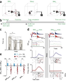
Reward biases spontaneous neural reactivation during sleep

Sleep restores an optimal computational regime in cortical networks

Sleep loss diminishes hippocampal reactivation and replay
Change history, 18 july 2017.
In the version of this article initially published online, the abstract read "casual neuron–behavior relationship" instead of "causal neuron–behavior relationship." The error has been corrected in the print, PDF and HTML versions of this article.
31 July 2017
In the version of this article initially published online, the x -axis label for the righthand column in each graph in Figure 6b read BMI 1Early ; it should have read BMI 2Early . The error has been corrected in the print, PDF and HTML versions of this article.
Yin, H.H. et al. Dynamic reorganization of striatal circuits during the acquisition and consolidation of a skill. Nat. Neurosci. 12 , 333–341 (2009).
CAS PubMed PubMed Central Google Scholar
Dayan, E. & Cohen, L.G. Neuroplasticity subserving motor skill learning. Neuron 72 , 443–454 (2011).
Tumer, E.C. & Brainard, M.S. Performance variability enables adaptive plasticity of 'crystallized' adult birdsong. Nature 450 , 1240–1244 (2007).
CAS PubMed Google Scholar
Shmuelof, L. & Krakauer, J.W. Are we ready for a natural history of motor learning? Neuron 72 , 469–476 (2011).
Peters, A.J., Chen, S.X. & Komiyama, T. Emergence of reproducible spatiotemporal activity during motor learning. Nature 510 , 263–267 (2014).
Ganguly, K. & Carmena, J.M. Emergence of a stable cortical map for neuroprosthetic control. PLoS Biol. 7 , e1000153 (2009).
PubMed PubMed Central Google Scholar
Huber, D. et al. Multiple dynamic representations in the motor cortex during sensorimotor learning. Nature 484 , 473–478 (2012).
Ganguly, K., Dimitrov, D.F., Wallis, J.D. & Carmena, J.M. Reversible large-scale modification of cortical networks during neuroprosthetic control. Nat. Neurosci. 14 , 662–667 (2011).
Abbott, L.F., DePasquale, B. & Memmesheimer, R.M. Building functional networks of spiking model neurons. Nat. Neurosci. 19 , 350–355 (2016).
Lee, D., Seo, H. & Jung, M.W. Neural basis of reinforcement learning and decision making. Annu. Rev. Neurosci. 35 , 287–308 (2012).
Clancy, K.B., Koralek, A.C., Costa, R.M., Feldman, D.E. & Carmena, J.M. Volitional modulation of optically recorded calcium signals during neuroprosthetic learning. Nat. Neurosci. 17 , 807–809 (2014).
Tononi, G. & Cirelli, C. Sleep and the price of plasticity: from synaptic and cellular homeostasis to memory consolidation and integration. Neuron 81 , 12–34 (2014).
Diekelmann, S. & Born, J. The memory function of sleep. Nat. Rev. Neurosci. 11 , 114–126 (2010).
Genzel, L., Kroes, M.C., Dresler, M. & Battaglia, F.P. Light sleep versus slow wave sleep in memory consolidation: a question of global versus local processes? Trends Neurosci. 37 , 10–19 (2014).
Cramer, S.C. et al. Motor cortex activation is preserved in patients with chronic hemiplegic stroke. Ann. Neurol. 52 , 607–616 (2002).
PubMed Google Scholar
Marshall, L. & Born, J. The contribution of sleep to hippocampus-dependent memory consolidation. Trends Cogn. Sci. 11 , 442–450 (2007).
Wilson, M.A. & McNaughton, B.L. Reactivation of hippocampal ensemble memories during sleep. Science 265 , 676–679 (1994).
Nere, A., Hashmi, A., Cirelli, C. & Tononi, G. Sleep-dependent synaptic down-selection (I): modeling the benefits of sleep on memory consolidation and integration. Front. Neurol. 4 , 143 (2013).
Jarosiewicz, B. et al. Functional network reorganization during learning in a brain-computer interface paradigm. Proc. Natl. Acad. Sci. USA 105 , 19486–19491 (2008).
Koralek, A.C., Jin, X., Long, J.D. II, Costa, R.M. & Carmena, J.M. Corticostriatal plasticity is necessary for learning intentional neuroprosthetic skills. Nature 483 , 331–335 (2012).
Taylor, D.M., Tillery, S.I. & Schwartz, A.B. Direct cortical control of 3D neuroprosthetic devices. Science 296 , 1829–1832 (2002).
Moritz, C.T., Perlmutter, S.I. & Fetz, E.E. Direct control of paralyzed muscles by cortical neurons. Nature 456 , 639–642 (2008).
Gulati, T., Ramanathan, D.S., Wong, C.C. & Ganguly, K. Reactivation of emergent task-related ensembles during slow-wave sleep after neuroprosthetic learning. Nat. Neurosci. 17 , 1107–1113 (2014).
Gulati, T. et al. Robust neuroprosthetic control from the stroke perilesional cortex. J. Neurosci. 35 , 8653–8661 (2015).
Fetz, E.E. Volitional control of neural activity: implications for brain-computer interfaces. J. Physiol. (Lond.) 579 , 571–579 (2007).
CAS Google Scholar
Koralek, A.C., Costa, R.M. & Carmena, J.M. Temporally precise cell-specific coherence develops in corticostriatal networks during learning. Neuron 79 , 865–872 (2013).
Orsborn, A.L. et al. Closed-loop decoder adaptation shapes neural plasticity for skillful neuroprosthetic control. Neuron 82 , 1380–1393 (2014).
Mitchell, J.F., Sundberg, K.A. & Reynolds, J.H. Spatial attention decorrelates intrinsic activity fluctuations in macaque area V4. Neuron 63 , 879–888 (2009).
Watson, B.O., Levenstein, D., Greene, J.P., Gelinas, J.N. & Buzsáki, G. Network homeostasis and state dynamics of neocortical sleep. Neuron 90 , 839–852 (2016).
Peyrache, A., Khamassi, M., Benchenane, K., Wiener, S.I. & Battaglia, F.P. Replay of rule-learning related neural patterns in the prefrontal cortex during sleep. Nat. Neurosci. 12 , 919–926 (2009).
Ramanathan, D.S., Gulati, T. & Ganguly, K. Sleep-dependent reactivation of ensembles in motor cortex promotes skill consolidation. PLoS Biol. 13 , e1002263 (2015).
Lansink, C.S., Goltstein, P.M., Lankelma, J.V., McNaughton, B.L. & Pennartz, C.M. Hippocampus leads ventral striatum in replay of place-reward information. PLoS Biol. 7 , e1000173 (2009).
de Lavilléon, G., Lacroix, M.M., Rondi-Reig, L. & Benchenane, K. Explicit memory creation during sleep demonstrates a causal role of place cells in navigation. Nat. Neurosci. 18 , 493–495 (2015).
Singer, A.C. & Frank, L.M. Rewarded outcomes enhance reactivation of experience in the hippocampus. Neuron 64 , 910–921 (2009).
Churchland, M.M. et al. Stimulus onset quenches neural variability: a widespread cortical phenomenon. Nat. Neurosci. 13 , 369–378 (2010).
Song, W. & Giszter, S.F. Adaptation to a cortex-controlled robot attached at the pelvis and engaged during locomotion in rats. J. Neurosci. 31 , 3110–3128 (2011).
Miyamoto, D. et al. Top-down cortical input during NREM sleep consolidates perceptual memory. Science 352 , 1315–1318 (2016).
Chuong, A.S. et al. Noninvasive optical inhibition with a red-shifted microbial rhodopsin. Nat. Neurosci. 17 , 1123–1129 (2014).
Steriade, M., Nuñez, A. & Amzica, F. A novel slow (<1 Hz) oscillation of neocortical neurons in vivo: depolarizing and hyperpolarizing components. J. Neurosci. 13 , 3252–3265 (1993).
Yang, G. et al. Sleep promotes branch-specific formation of dendritic spines after learning. Science 344 , 1173–1178 (2014).
de Vivo, L. et al. Ultrastructural evidence for synaptic scaling across the wake/sleep cycle. Science 355 , 507–510 (2017).
Maret, S., Faraguna, U., Nelson, A.B., Cirelli, C. & Tononi, G. Sleep and waking modulate spine turnover in the adolescent mouse cortex. Nat. Neurosci. 14 , 1418–1420 (2011).
Gupta, A.S., van der Meer, M.A., Touretzky, D.S. & Redish, A.D. Hippocampal replay is not a simple function of experience. Neuron 65 , 695–705 (2010).
O'Doherty, J.P., Cockburn, J. & Pauli, W.M. Learning, reward, and decision making. Annu. Rev. Psychol. 68 , 73–100 (2017).
Schultz, W. Behavioral theories and the neurophysiology of reward. Annu. Rev. Psychol. 57 , 87–115 (2006).
Ishii, S., Yoshida, W. & Yoshimoto, J. Control of exploitation-exploration meta-parameter in reinforcement learning. Neural Netw. 15 , 665–687 (2002).
Wallstrom, G., Liebner, J. & Kass, R.E. An implementation of Bayesian adaptive regression splines (BARS) in C with S and R Wrappers. J. Stat. Softw. 26 , 1–21 (2008).
Mitra, P. & Bokil, H. Observed Brain Dynamics (Oxford University Press, 2008).
Download references
Acknowledgements
This work was supported by awards from the Department of Veterans Affairs, Veterans Health Administration (VA Merit: 1I01RX001640 to K.G., VA CDA 1IK2BX003308 to D.S.R.); the National Institute of Neurological Disorders and Stroke (1K99NS097620 to T.G. and 5K02NS093014 to K.G.); the American Heart/Stroke Association (15POST25510020 to T.G.); the Burroughs Wellcome Fund (1009855 to K.G.); and start-up funds from the SFVAMC, NCIRE and UCSF Department of Neurology (to K.G.).
Author information
Authors and affiliations.
Neurology and Rehabilitation Service, San Francisco Veterans Affairs Medical Center, San Francisco, California, USA
Tanuj Gulati, Ling Guo, Dhakshin S Ramanathan, Anitha Bodepudi & Karunesh Ganguly
Department of Neurology, University of California-San Francisco, San Francisco, California, USA
Tanuj Gulati, Ling Guo, Anitha Bodepudi & Karunesh Ganguly
Center for Neural Engineering and Prostheses, University of California-Berkeley and University of California-San Francisco, California, USA
Tanuj Gulati, Ling Guo, Dhakshin S Ramanathan & Karunesh Ganguly
Department of Psychiatry, San Francisco Veterans Affairs Medical Center, San Francisco, California, USA
Dhakshin S Ramanathan
Department of Psychiatry, University of California-San Francisco, San Francisco, California, USA
You can also search for this author in PubMed Google Scholar
Contributions
T.G. and K.G. conceived of the experiments. L.G. and T.G. performed surgical procedures and collected the data. A.B., D.S.R. and T.G. analyzed the data. T.G. and K.G. wrote the manuscript. L.G. and D.S.R. edited the manuscript.
Corresponding author
Correspondence to Karunesh Ganguly .
Ethics declarations
Competing interests.
The authors declare no competing financial interests.
Integrated supplementary information
Supplementary figure 1 modulations of tr d neurons are not significantly high during random time points in sleep..
a , Mean modulation of all TR D and TR I neurons at randomly picked times during Sleep post . For this analysis, snippets of activity (50 ms window of spiking activity that was then binned at 5 ms resolution) were randomly sampled from all the reactivation times. b , Scatter plots showing the modulation depth for all the individual TR D and TR I (mean in solid line ± s.e.m. in box; unpaired t test t 121 = 0.69, P = 0.49).
Supplementary Figure 2 Depth modulation during sleep reactivations predicts rescaling of task–related firing rate during BMI 2 .
MD reactivation from Sleep post (in Fig 2c ) are compared to changes in modulation from BMI 1 to BMI 2 for both TR D and TR I neurons (linear regression R 2 = 0.17, P < 10 -5 ).
Supplementary Figure 3 Characteristics of OPTO UP and OPTO DOWN experiments.
a , Comparison of the total number of 100 ms optogenetic stimulation periods for OPTO UP and OPTO DOWN experiments (mean in solid line ± s.e.m. in box; color convention same as Fig 5 ; unpaired t test t 17 = 0.99, P = 0.33). b , Comparison of the proportion of total time that the LED was turned on for the respective Sleep post during the OPTO UP and OPTO DOWN experiments (mean in solid line ± s.e.m. in box; color convention same as Fig 5; unpaired t test t 17 = 2.07, P = 0.054).
Supplementary Figure 4 Sleep durations in optogenetic experiments.
Comparison of the total sleep durations for Sleep pre and Sleep post during the OPTO UP , OPTO DOWN and OPTO OFF experiments (mean in solid line ± s.e.m. in box, one-way ANOVA, F 5,48 = 0.92, P = 0.47; post hoc t test shows no significant difference between any pairwise comparison).
Supplementary Figure 5 PC weights for PCA based reactivation analysis.
Examples of the first principal components from two separate experiments. Notably, TR D and TR I neurons both had non-zero weights ( TR D enclosed in red box).
Supplementary information
Supplementary text and figures.
Supplementary Figures 1–5. (PDF 522 kb)
Supplementary Methods Checklist (PDF 539 kb)
Rights and permissions.
Reprints and permissions
About this article
Cite this article.
Gulati, T., Guo, L., Ramanathan, D. et al. Neural reactivations during sleep determine network credit assignment. Nat Neurosci 20 , 1277–1284 (2017). https://doi.org/10.1038/nn.4601
Download citation
Received : 22 June 2016
Accepted : 23 May 2017
Published : 10 July 2017
Issue Date : 01 September 2017
DOI : https://doi.org/10.1038/nn.4601
Share this article
Anyone you share the following link with will be able to read this content:
Sorry, a shareable link is not currently available for this article.
Provided by the Springer Nature SharedIt content-sharing initiative
This article is cited by
Spindle oscillations in communicating axons within a reconstituted hippocampal formation are strongest in ca3 without thalamus.
- Mengke Wang
- Samuel B. Lassers
- Gregory J. Brewer
Scientific Reports (2024)
Probing pathways by which rhynchophylline modifies sleep using spatial transcriptomics
- Maria Neus Ballester Roig
- Tanya Leduc
- Valérie Mongrain
Biology Direct (2023)
Emergence of cortical network motifs for short-term memory during learning
- Xin Wei Chia
- Jian Kwang Tan
- Hiroshi Makino
Nature Communications (2023)
Emergence of task-related spatiotemporal population dynamics in transplanted neurons
- Harman Ghuman
- Kyungsoo Kim
- Karunesh Ganguly
Cortical–hippocampal coupling during manifold exploration in motor cortex
- Jaekyung Kim
- Abhilasha Joshi
Nature (2023)
Quick links
- Explore articles by subject
- Guide to authors
- Editorial policies
Sign up for the Nature Briefing newsletter — what matters in science, free to your inbox daily.

Credit assignment for trained neural networks based on Koopman operator theory
- Published: 04 September 2023
- Volume 18 , article number 181324 , ( 2024 )
Cite this article

- Zhen Liang 1 ,
- Changyuan Zhao 2 ,
- Wanwei Liu 3 ,
- Bai Xue 2 ,
- Wenjing Yang 1 &
- Zhengbin Pang 3
26 Accesses
Explore all metrics
This is a preview of subscription content, log in via an institution to check access.
Access this article
Subscribe and save.
- Get 10 units per month
- Download Article/Chapter or eBook
- 1 Unit = 1 Article or 1 Chapter
- Cancel anytime
Price includes VAT (Russian Federation)
Instant access to the full article PDF.
Rent this article via DeepDyve
Institutional subscriptions
Dahnert M, Hou J, Nießner M, et al. Panoptic 3D scene reconstruction from a single RGB image. In: Proceedings of the 35th Neural Information Processing Systems. 2021, 8282–8293
Tian Y, Yang W, Wang J. Image fusion using a multi-level image decomposition and fusion method. Applied Optics, 2021, 60(24): 7466–7479
Article Google Scholar
Liang Z, Cai Z, Li M, et al. Parallel gym gazebo: a scalable parallel robot deep reinforcement learning platform. In: Proceedings of the 31st IEEE International Conference on Tools with Artificial Intelligence. 2019, 206–213
Minsky M. Steps toward artificial intelligence. Proceedings of the IRE, 1961, 49(1): 8–30
Article MathSciNet Google Scholar
Whitney H. Differentiable manifolds. Annals of Mathematics, 1936, 37(3): 645–680
Article MathSciNet MATH Google Scholar
Takens F. Detecting strange attractors in turbulence. In: Rand D, Young L S, eds. Dynamical Systems and Turbulence, Warwick 1980. Berlin, Heidelberg: Springer, 1981, 366–381
Chapter Google Scholar
Kutz J N, Brunton S L, Brunton B W, Proctor J L. Dynamic Mode Decomposition: Data-Driven Modeling of Complex Systems. Philadelphia: Society for Industrial and Applied Mathematics, 2016
Book MATH Google Scholar
Lecun Y, Bottou L, Bengio Y, Haffner P. Gradient-based learning applied to document recognition. Proceedings of the IEEE, 1998, 86(11): 2278–2324
Download references
Acknowledgements
This work was supported by the National Natural Science Foundation of China (Grant Nos. 61872371, 61836005 and 62032024) and the CAS Pioneer Hundred Talents Program.
Author information
Authors and affiliations.
Institute for Quantum Information & State Key Laboratory of High Performance Computing, National University of Defense Technology, Changsha, 410000, China
Zhen Liang & Wenjing Yang
Institute of Software, Chinese Academy of Sciences, Beijing, 100190, China
Changyuan Zhao & Bai Xue
College of Computer Science and Technology, National University of Defense Technology, Changsha, 410000, China
Wanwei Liu & Zhengbin Pang
You can also search for this author in PubMed Google Scholar
Corresponding author
Correspondence to Wanwei Liu .
Ethics declarations
Competing interests The authors declare that they have no competing interests or financial conflicts to disclose.
Electronic Supplementary Material
Credit assignment for trained neural networks based on koopman operator theory, rights and permissions.
Reprints and permissions
About this article
Liang, Z., Zhao, C., Liu, W. et al. Credit assignment for trained neural networks based on Koopman operator theory. Front. Comput. Sci. 18 , 181324 (2024). https://doi.org/10.1007/s11704-023-2629-4
Download citation
Received : 16 October 2022
Accepted : 09 May 2023
Published : 04 September 2023
DOI : https://doi.org/10.1007/s11704-023-2629-4
Share this article
Anyone you share the following link with will be able to read this content:
Sorry, a shareable link is not currently available for this article.
Provided by the Springer Nature SharedIt content-sharing initiative
- Find a journal
- Publish with us
- Track your research
Credit Assignment Through Broadcasting a Global Error Vector
Part of Advances in Neural Information Processing Systems 34 (NeurIPS 2021)
David Clark, L F Abbott, Sueyeon Chung
Backpropagation (BP) uses detailed, unit-specific feedback to train deep neural networks (DNNs) with remarkable success. That biological neural circuits appear to perform credit assignment, but cannot implement BP, implies the existence of other powerful learning algorithms. Here, we explore the extent to which a globally broadcast learning signal, coupled with local weight updates, enables training of DNNs. We present both a learning rule, called global error-vector broadcasting (GEVB), and a class of DNNs, called vectorized nonnegative networks (VNNs), in which this learning rule operates. VNNs have vector-valued units and nonnegative weights past the first layer. The GEVB learning rule generalizes three-factor Hebbian learning, updating each weight by an amount proportional to the inner product of the presynaptic activation and a globally broadcast error vector when the postsynaptic unit is active. We prove that these weight updates are matched in sign to the gradient, enabling accurate credit assignment. Moreover, at initialization, these updates are exactly proportional to the gradient in the limit of infinite network width. GEVB matches the performance of BP in VNNs, and in some cases outperforms direct feedback alignment (DFA) applied in conventional networks. Unlike DFA, GEVB successfully trains convolutional layers. Altogether, our theoretical and empirical results point to a surprisingly powerful role for a global learning signal in training DNNs.
Name Change Policy
Requests for name changes in the electronic proceedings will be accepted with no questions asked. However name changes may cause bibliographic tracking issues. Authors are asked to consider this carefully and discuss it with their co-authors prior to requesting a name change in the electronic proceedings.
Use the "Report an Issue" link to request a name change.
Credit Assignment for Trained Neural Networks Based on Koopman Operator Theory

Credit assignment problem of neural networks refers to evaluating the credit of each network component to the final outputs. For an untrained neural network, approaches to tackling it have made great contributions to parameter update and model revolution during the training phase. This problem on trained neural networks receives rare attention, nevertheless, it plays an increasingly important role in neural network patch, specification and verification. Based on Koopman operator theory, this paper presents an alternative perspective of linear dynamics on dealing with the credit assignment problem for trained neural networks. Regarding a neural network as the composition of sub-dynamics series, we utilize step-delay embedding to capture snapshots of each component, characterizing the established mapping as exactly as possible. To circumvent the dimension-difference problem encountered during the embedding, a composition and decomposition of an auxiliary linear layer, termed minimal linear dimension alignment, is carefully designed with rigorous formal guarantee. Afterwards, each component is approximated by a Koopman operator and we derive the Jacobian matrix and its corresponding determinant, similar to backward propagation. Then, we can define a metric with algebraic interpretability for the credit assignment of each network component. Moreover, experiments conducted on typical neural networks demonstrate the effectiveness of the proposed method.
Please sign up or login with your details
Generation Overview
AI Generator calls
AI Video Generator calls
AI Chat messages
Genius Mode messages
Genius Mode images
AD-free experience
Private images
- Includes 500 AI Image generations, 1750 AI Chat Messages, 30 AI Video generations, 60 Genius Mode Messages and 60 Genius Mode Images per month. If you go over any of these limits, you will be charged an extra $5 for that group.
- For example: if you go over 500 AI images, but stay within the limits for AI Chat and Genius Mode, you'll be charged $5 per additional 500 AI Image generations.
- Includes 100 AI Image generations and 300 AI Chat Messages. If you go over any of these limits, you will have to pay as you go.
- For example: if you go over 100 AI images, but stay within the limits for AI Chat, you'll have to reload on credits to generate more images. Choose from $5 - $1000. You'll only pay for what you use.
Out of credits
Refill your membership to continue using DeepAI
Share your generations with friends
IMAGES
VIDEO
COMMENTS
The credit assignment problem (CAP) is a fundamental challenge in reinforcement learning. It arises when an agent receives a reward for a particular action, but the agent must determine which of its previous actions led to the reward. In reinforcement learning, an agent applies a set of actions in an environment to maximize the overall reward.
An excerpt from Box 1 in the article "A deep learning framework for neuroscience", by Blake A. Richards et. al. (among the authors is Yoshua Bengio):The concept of credit assignment refers to the problem of determining how much 'credit' or 'blame' a given neuron or synapse should get for a given outcome.
Credit Assignment in Neural Networks through Deep Feedback Control. 2. Credit assignment (CA) 2 ... Optimal credit assignment without the need for strict alignment Intimate connection with cortical pyramidal neurons 22. Thank you! 23 Javier García Ordóñez Pau Vilimelis Aceituno
Here, we introduce Deep Feedback Control (DFC), a new learning method that uses a feedback controller to drive a deep neural network to match a desired output target and whose control signal can be used for credit assignment. The resulting learning rule is fully local in space and time and approximates Gauss-Newton optimization for a wide range ...
Credit Assignment in Neural Networks through Deep Feedback Control Alexander Meulemans, Matilde Tristany Farinha , Javier García Ordóñez, ... (BP) algorithm [1, 2, 3] is currently the gold standard to perform credit assignment (CA) in deep neural networks. Although deep learning was inspired by biological neural
2 The biology of neural networks: a few features for the sake of non-biologists; 3 The dynamics of neural networks: a stochastic approach; 4 Hebbian models of associative memory; 5 Temporal sequences of patterns; 6 The problem of learning in neural networks; 7 Learning dynamics in 'visible' neural networks; 8 Solving the problem of credit ...
A biologically plausible neural network for local supervision in cortical microcircuits, 2020. Bengio [2014] Yoshua Bengio. How auto-encoders could provide credit assignment in deep networks via target propagation. arXiv preprint arXiv:1407.7906, 2014. Lee et al. [2015] Dong-Hyun Lee, Saizheng Zhang, Asja Fischer, and Yoshua Bengio.
Here, we introduce Deep Feedback Control (DFC), a new learning method. that uses a feedback controller to drive a deep neural network to match a desired. output target and whose control signal can ...
Structural credit assignment in neural networks is a long-standing problem, with a variety of alternatives to backpropagation proposed to allow for local training of nodes. One of the early strategies was to treat each node as an agent and use a reinforcement learning method called REINFORCE to update each node locally with only a global reward ...
the learning credit assignment of neural networks. The spike is intimately related to the concept of network compression [10,17,18], where not all resources of con-nections are used in a task. This parameter allows one to identify very important weights and further evaluate remaining capacities for learning new tasks [19]. A recent
Assigning credit or blame for each of those actions individually is known as the (temporal) Credit Assignment Problem (CAP) . The CAP is particularly relevant for real-world tasks, where we need to learn effective policies from small, limited training datasets. ... To train the neural network, InferNet distributes the final delayed reward among ...
In artificial neural networks, the three components specified by design are the objective functions, the learning rules and the architectures. ... The concept of credit assignment refers to the ...
temporal credit assignment, but in the opposite direction from this work: specifying temporal credit assignment as a structural credit assignment problem [4]. Once we use RL agents as nodes, which have stochastic policies, there is a clear connection to the work on stochastic neural networks. Much of this work has looked at networks with stochastic
In reinforcement learning (RL), an agent interacts with an environment in time steps. On each time step, the agent takes an action in a certain state and the environment emits a percept or perception, which is composed of a reward and an observation, which, in the case of fully-observable MDPs, is the next state (of the environment and the agent).The goal of the agent is to maximise the reward ...
the number of units in the network (Rezende et al., 2014). This drives the hypothesis that learning in the brain must rely on additional structures beyond a global reward signal. In artificial neural networks (ANNs), credit assignment is performed with gradient-based methods
The foundation of curriculum learning is that deep neural networks can generalize well between different environments. However, it only holds if the network architecture, the designed curriculum, and the task fit perfectly together. We refer to those methods as model-free credit assignments in the following sections.
Learning in hierarchical neural networks requires credit assignment. • Credit assignment is difficult if regular inputs mix with credit signals. • Dendritic mechanisms provide potential means of distinguishing credit signals. • Evidence supports credit assignment in apical dendrites of pyramidal neurons.
Spiking neural networks (SNNs) take inspiration from the brain to enable energy-efficient computations. ... In addition, one can observe how, during the backward pass using BPTT, credit assignment ...
CBMM researchers Giorgia Dellaferrera and Gabriel Kreiman discuss their latest paper, published in Proceedings of Machine Learning Research 2022 (https://pro...
A fundamental goal of learning is to establish neural patterns that cause desired behaviors. This paper demonstrates that sleep-dependent processing is required for credit assignment and the ...
Credit Assignment for Trained Neural Networks Based on Koopman Operator Theory. Rights and permissions. Reprints and permissions. About this article. Cite this article. Liang, Z., Zhao, C., Liu, W. et al. Credit assignment for trained neural networks based on Koopman operator theory.
Backpropagation (BP) uses detailed, unit-specific feedback to train deep neural networks (DNNs) with remarkable success. That biological neural circuits appear to perform credit assignment, but cannot implement BP, implies the existence of other powerful learning algorithms. Here, we explore the extent to which a globally broadcast learning ...
Here, we introduce Deep Feedback Control (DFC), a new learning method that uses a feedback controller to drive a deep neural network to match a desired output target and whose control signal can be used for credit assignment. The resulting learning rule is fully local in space and time and approximates Gauss-Newton optimization for a wide range ...
Credit assignment problem of neural networks refers to evaluating the credit of each network component to the final outputs. For an untrained neural network, approaches to tackling it have made great contributions to parameter update and model revolution during the training phase. This problem on trained neural networks receives rare attention ...
Credit assignment problem of neural networks refers to evaluating the credit of each network component to the final outputs. For an untrained neural network, approaches to tackling it have made great contributions to parameter update and model revolution during the training phase. This problem on trained neural networks receives rare attention, nevertheless, it plays an increasingly important ...