Dependent and independent samples
What is the difference between a dependent sample and an independent sample? And why is it important to know the difference? Whether the data at hand are from a dependent or an independent sample determines which hypothesis test is used.
If your data are independent, for example, an independent samples t-test or an ANOVA without repeated measures is calculated. If your data are dependent, a t-test for dependent samples or an ANOVA with repeated measures is calculated.


Example independent and dependent variable
Let's say you want to find out whether holidays have an effect on people's stress levels. To find out, you have created a small online survey on datatab.net that allows you to measure people's stress levels. In the survey, you ask people about their stress levels before and after their holiday. You now have two options:

In the left case you would have an independent sample, because the people you interviewed before the holiday have nothing to do with the people you interviewed after the holiday.
In the right case you would have a dependent sample, you would interview people before the holiday and interview the same people after the holiday, so the measures are always available in pairs. In this case, this is the preferred solution for this research question!
Dependent sample
In a dependent sample, the measures are related. For example, if you take a sample of people who have had a knee operation and interview them before and after the operation, this is a dependent sample. This is because the same person was interviewed at two different times.
Of course, there does not necessarily need to be a before-and-after relationship to be studied.
For example, if you want to investigate whether a new baseball bat has an effect on batting performance, and the same people play once with the old bat and once with the new one, then you have a dependent sample. In this case, the measurements are also available in pairs, each player has used both bats, so there are two measurements for each player.
And it does not have to be the same person. For example, if you wanted to find out whether, in a relationship between men and women, women do more gardening than men, you would also have a dependent sample. You would have two measures that always go together in pairs, always one woman and one man.

Independent sample
In independent samples, the values come from two or more different groups. For example, if the men's group and the women's group are asked about their income, independent samples exist. In this case, a person from one sample cannot be assigned to a person from the other sample.
More than two dependent or independent samples
Of course, in the case of independent and dependent sampling, there can be more than two samples. The important thing is that in the case of independent sampling, the individual groups or samples have nothing to do with each other, and in the case of dependent sampling, a respondent appears in all groups.
Hypothesis testing for dependent and independent samples
In general, there is always a hypothesis test for independent samples and a counterpart for dependent samples. Instead of the term dependent and independent , paired and unpaired are often used in the case of analysis of variance with and without repeated measures, as well as in the case of the t-test.
| Dependent sample | Independent sample |
|---|---|
In DATAtab you can choose with one click whether you want to calculate the respective hypothesis test for dependent or independent samples.

Depending on the format in which you insert your data, a variant is pre-selected. Usually, a series is a respondent or, more generally, a case. Therefore, metric values that are in a series are initially considered dependent.
If a metric and a categorical variable are clicked, the respective independent test is automatically selected.

Statistics made easy
- many illustrative examples
- ideal for exams and theses
- statistics made easy on 412 pages
- 5rd revised edition (April 2024)
- Only 8.99 €

"Super simple written"
"It could not be simpler"
"So many helpful examples"

Cite DATAtab: DATAtab Team (2024). DATAtab: Online Statistics Calculator. DATAtab e.U. Graz, Austria. URL https://datatab.net
Dependent t-test for paired samples (cont...)
What hypothesis is being tested.
The dependent t-test is testing the null hypothesis that there are no differences between the means of the two related groups. If we get a statistically significant result, we can reject the null hypothesis that there are no differences between the means in the population and accept the alternative hypothesis that there are differences between the means in the population. We can express this as follows:
H 0 : µ 1 = µ 2
H A : µ 1 ≠ µ 2
What is the advantage of a dependent t-test over an independent t-test?
Before we answer this question, we need to point out that you cannot choose one test over the other unless your study design allows it. What we are discussing here is whether it is advantageous to design a study that uses one set of participants whom are measured twice or two separate groups of participants measured once each. The major advantage of choosing a repeated-measures design (and therefore, running a dependent t-test) is that you get to eliminate the individual differences that occur between participants – the concept that no two people are the same – and this increases the power of the test. What this means is that if you are more likely to detect a (statistically significant) difference, if one does exist, using the dependent t-test versus the independent t-test.
Can the dependent t-test be used to compare different participants?
Yes, but this does not happen very often. You can use the dependent t-test instead of using the usual independent t-test when each participant in one of the independent groups is closely related to another participant in the other group on many individual characteristics. This approach is called a "matched-pairs" design. The reason we might want to do this is that the major advantage of running a within-subject (repeated-measures) design is that you get to eliminate between-groups variation from the equation (each individual is unique and will react slightly differently than someone else), thereby increasing the power of the test. Hence, the reason why we use the same participants – we expect them to react in the same way as they are, after all, the same person. The most obvious case of when a "matched-pairs" design might be implemented is when using identical twins. Effectively, you are choosing parameters to match your participants on, which you believe will result in each pair of participants reacting in a similar way.
How do I report the result of a dependent t-test?
You need to report the test as follows:

where df is N – 1, where N = number of participants.

Should I report confidence levels?
Confidence intervals (CI) are a useful statistic to include because they indicate the direction and size of a result. It is common to report 95% confidence intervals, which you will most often see reported as 95% CI. Programmes such as SPSS Statistics will automatically calculate these confidence intervals for you; otherwise, you need to calculate them by hand. You will want to report the mean and 95% confidence interval for the difference between the two related groups.
If you wish to run a dependent t-test in SPSS Statistics, you can find out how to do this in our Dependent T-Test guide.
- Skip to secondary menu
- Skip to main content
- Skip to primary sidebar
Statistics By Jim
Making statistics intuitive
Paired T Test: Definition & When to Use It
By Jim Frost 5 Comments
What is a Paired T Test?
Use a paired t-test when each subject has a pair of measurements, such as a before and after score. A paired t-test determines whether the mean change for these pairs is significantly different from zero. This test is an inferential statistics procedure because it uses samples to draw conclusions about populations.
Paired t tests are also known as a paired sample t-test or a dependent samples t test. These names reflect the fact that the two samples are paired or dependent because they contain the same subjects. Conversely, an independent samples t test contains different subjects in the two samples.

For example, you gather a random sample of people, give them a pretest, administer a training program, and then perform a posttest. Each subject has a paired pretest and posttest score, and you want to determine whether there is significant improvement between the tests.
Or, perhaps you have a sample of wood boards, and you paint half of each board with one paint and the other half with the other paint. Then, you measure the paint durability for both types of paint on all the boards. Each board has two paint durability scores, and you want to determine whether the two paints have different durability.
In both cases, you have the same subjects/items in both groups. Each subject has a pair of measurements. A paired t-test determines whether the mean difference of these pairs equals zero (no effect ).
In this article, you’ll learn about the hypotheses, assumptions, and how to interpret the results for paired t tests.
Related post : Difference between Descriptive and Inferential Statistics
Paired T Test Hypotheses
Paired t tests have the following hypotheses:
- Null hypothesis: The mean of the paired differences equals zero in the population .
- Alternative hypothesis : The mean of the paired differences does not equal zero in the population.
If the p-value is less than your significance level (e.g., 0.05), you can reject the null hypothesis. Your sample provides strong enough evidence to conclude that the mean paired difference does not equal zero in the population. Learn more about the Null Hypothesis: Definition, Rejecting & Examples .
Notice how the hypotheses reflect the paired sample nature of this t-test. This test assesses the mean difference between the pairs.
Related post : How to Interpret P Values
Paired T Test Assumptions
For reliable paired sample t-test results, your data should satisfy the following assumptions.
You have a random sample with independent subjects
Drawing a random sample from the population you are studying helps ensure that your data represent the population. Representative samples are vital when drawing inferences about the population. If your data do not represent the population, your analysis results will not be valid for that population.
When drawing a random sample, each item or person must have the same probability of being selected.
Related post : Populations, Parameters, and Samples in Inferential Statistics
Dependent Samples
Paired sample t-tests use the same people or items in both groups. These are dependent samples, also known as paired samples.
Dependent samples can increase the statistical power of your analyses. To learn why, read my post about Independent and Dependent Samples .
It’s important to distinguish between independent subjects when drawing a random sample and dependent samples when measuring. When choosing the subjects, selecting one must not affect the probability of choosing the others. However, after selecting your subjects, they will all be in both groups. In this manner, you have independent subjects but dependent samples.
If the two groups contain different subjects, use an independent samples t test instead.
Your data must be continuous
T tests require continuous data . Continuous variables can take on any numeric value. Values can be meaningfully divided into smaller increments, including fractional and decimal values. Typically, you measure continuous variables on a scale. For example, weight, temperature, and height are continuous data.
If you don’t have continuous data, you’ll need to use a different type of hypothesis test. To learn more, read my post, Comparing Hypothesis Tests for Continuous, Binary, and Count Data .
Data should follow a normal distribution or have a sample size larger than 20
All t-tests assume that your data follow the normal distribution . For a paired t test, the normality assumption applies to the distribution of paired differences rather than raw test scores. However, you can waive this assumption for mildly skewed data when your distribution is unimodal and the sample size is large enough thanks to the central limit theorem.
For a paired sample t test, if you have at least 20 subjects, your test results will be reliable even when your data are skewed. However, when you have a smaller sample size, nonnormal data can cause the test results to be unreliable.
Be sure to check for outliers because they can throw off the results.
Related posts : Central Limit Theorem , Skewed Distributions and 5 Ways to Find Outliers .
Paired T Test Example
For example, imagine we have a training program and administer a pretest and posttest to the same sample of students. Consequently, each student has a pair of test scores. We need to determine whether the average change for the pairs of scores is different from zero.
Here is what the data look like in the datasheet. Note that the analysis does not use the subject’s ID number.

Here’s the deciding characteristic for when you should use paired t tests versus an independent samples t test. Does it make sense to assess the difference within a row? In other words, does each row correspond to one person or item? Are the samples paired with each other?
For our dataset, each row in the dataset contains the same subject in the two measurement columns. Consequently, it makes sense to find the difference between the pairs of values. Because we have paired samples, each difference in a row represents how much a subject’s score changed after the training program. The paired t-test is the correct choice.
Conversely, if each row had contained different subjects, it would not make sense to subtract them. The change between the pretest for one subject and the posttest for another does not provide meaningful information. In that case, we’d need to perform an independent samples t test.
Interpreting the Results
Here’s how to read and report the results for a paired t test.

The output indicates that the mean for the Pretest is 97.06, and for the Posttest it is 107.83. The average difference between the paired pretest and posttest scores is -10.77. If the p-value is less than your significance level, the difference does not equal zero.
Because our p-value (0.002) for the paired sample t-test is less than the standard significance level of 0.05, we can reject the null hypothesis. The results are statistically significant. Our sample data support the notion that the average paired difference does not equal zero. Specifically, the Posttest mean is greater than the Pretest mean.
Learn more about Statistical Significance: Definition & Meaning .
The sample estimate of the difference (-10.77) is unlikely to equal the population difference. The confidence interval estimates that the actual population difference between the Pretest and Posttest is likely between -16.96 and -4.59.
The negative values reflect the fact that the Pretest has a lower mean than the Posttest (i.e., Pretest – Posttest < 0). The confidence interval excludes the zero (no difference between the paired samples) as a likely value, so we can conclude that the population difference does not equal zero.
If high scores are better, the paired sample t-test indicates that the Posttest scores are significantly better than the pretest scores.
To learn more about performing t-tests and how they work, read the following posts:
- T Test Overview
- One-Sample T-Test
- Two-Sample T-Test
- Running T Tests in Excel
- T-Values and T-Distributions
Share this:

Reader Interactions

August 17, 2022 at 11:35 pm
Hi! Our team is conducting a sensory evaluation of two cocoa blends. The blends vary in the amount of sweetener. A panel of 50 individuals will taste both blends and rate them based on a set criteria. In analyzing their ratings, which t-test is the most appropriate?

June 21, 2022 at 4:30 pm
I want to know if adding hood to a light bulb may change the brightness or not. So I measured the brightness from 30 light bulbs for group 1, then I add hoods to the same 30 light bulbs and measure the brightness again for group 2. In this setup, should I use paired sample t-test or two samples t-test to test if the mean brightness had no difference or not?
Could you please help on this?
Thank you, Mitch

June 21, 2022 at 11:17 pm
Because you’re using the same lightbulbs in both groups, you should use a paired sample t-test.

November 18, 2021 at 4:43 pm
One-Sample Statistics N Mean Std. Deviation Std. Error Mean Female 224 1.7098 .45486 .03039 Male 143 1.7273 .44693 .03737
One-Sample Test Test Value = 0 t df Sig. (2-tailed) Mean Difference 95% Confidence Interval of the Difference Lower Upper Female 56.260 223 .000 1.70982 1.6499 1.7697 Male 46.216 142 .000 1.72727 1.6534 1.8012
Therefore, Female show more of HTLV infection in comparison with Male.
is this true, could u kindly explain jim
November 21, 2021 at 8:24 pm
I really can’t interpret these results because I don’t know what the variables are measuring. Also, from what I can tell, there seems to be two different variables. And there seems to be some values missing as well and the lack of formatting is not helping.
Comments and Questions Cancel reply
Statistics Resources
- Excel - Tutorials
- Basic Probability Rules
- Single Event Probability
- Complement Rule
- Intersections & Unions
- Compound Events
- Levels of Measurement
- Independent and Dependent Variables
- Entering Data
- Central Tendency
- Data and Tests
- Displaying Data
- Discussing Statistics In-text
- SEM and Confidence Intervals
- Two-Way Frequency Tables
- Empirical Rule
- Finding Probability
- Accessing SPSS
- Chart and Graphs
- Frequency Table and Distribution
- Descriptive Statistics
- Converting Raw Scores to Z-Scores
- Converting Z-scores to t-scores
- Split File/Split Output
- Partial Eta Squared
- Downloading and Installing G*Power: Windows/PC
- Correlation
- Testing Parametric Assumptions
- One-Way ANOVA
- Two-Way ANOVA
- Repeated Measures ANOVA
- Goodness-of-Fit
- Test of Association
- Pearson's r
- Point Biserial
- Mediation and Moderation
- Simple Linear Regression
- Multiple Linear Regression
- Binomial Logistic Regression
- Multinomial Logistic Regression
- Independent Samples T-test
Dependent Samples T-test
- Testing Assumptions
- T-tests using SPSS
- T-Test Practice
- Predictive Analytics This link opens in a new window
- Quantitative Research Questions
- Null & Alternative Hypotheses
- One-Tail vs. Two-Tail
- Alpha & Beta
- Associated Probability
- Decision Rule
- Statement of Conclusion
- Statistics Group Sessions
The dependent samples t-test is used to compare the sample means from two related groups. This means that the scores for both groups being compared come from the same people. The purpose of this test is to determine if there is a change from one measurement (group) to the other.
Basic Hypotheses
Null: The mean difference between the two groups is not different from 0. Alternative: The mean difference between the two groups is different from 0.
Real-World Examples
- Is there an improvement in reading scores after participating in the Read Like a Pro course?
- Do people recall more words after learning a memorization strategy?
- Do people perform better when given praise or punishment?
- Is there a difference in how many miles a car can be driven when using AC versus having the windows down?
Reporting Results in APA Style
When reporting the results of the dependent-samples t-test, APA Style has very specific requirements on what information should be included. Below is the key information required for reporting the results of the. You want to replace the red text with the appropriate values from your output.
t (degrees of freedom) = the t statistic, p = p value.
Example : A dependent-samples t-test was run to determine if long-term recall improved with the introduction of the Say it Again memorization technique. The results showed that the average number of words recalled without this technique ( M = 13.5, SD = 2.4) was significantly less than the average number of words recalled with this technique ( M = 16.2, SD = 2.7), ( t (52) = 4.8, p < .001).
- When reporting the p-value, there are two ways to approach it. One is when the results are not significant. In that case, you want to report the p-value exactly: p = .24. The other is when the results are significant. In this case, you can report the p-value as being less than the level of significance: p < .05.
- The t statistic should be reported to two decimal places without a 0 before the decimal point: .36
- Degrees of freedom for this test are n - 1, where " n " represents the number of pairs in the sample. n can be found in the SPSS output.
Additional Resources
Laerd Statistics - Dependent T-test for Paired Samples guide Statistics Solutions - Paired Samples T-test
Was this resource helpful?
- << Previous: Independent Samples T-test
- Next: Testing Assumptions >>
- Last Updated: Jul 16, 2024 11:19 AM
- URL: https://resources.nu.edu/statsresources

t-test, Two Dependent Samples (Jump to: Lecture | Video )
Let's perform a dependent samples t-test: Researchers want to test a new anti-hunger weight loss pill. They have 10 people rate their hunger both before and after taking the pill. Does the pill do anything? Use alpha = 0.05
| Figure 1. |
|---|
| Steps for Dependent Samples t-Test |
|---|
| 1. Define Null and Alternative Hypotheses 2. State Alpha 3. Calculate Degrees of Freedom 4. State Decision Rule 5. Calculate Test Statistic 6. State Results 7. State Conclusion |
Let's begin.
1. Define Null and Alternative Hypotheses
| Figure 2. |
|---|
2. State Alpha
Alpha = 0.05
3. Calculate Degrees of Freedom
| Figure 3. |
|---|
4. State Decision Rule
Using an alpha of 0.05 with a two-tailed test with 9 degrees of freedom, we would expect our distribution to look something like this:
| Figure 4. |
|---|
Use the t-table to look up a two-tailed test with 9 degrees of freedom and an alpha of 0.05. We find a critical value of 2.2622. Thus, our decision rule for this two-tailed test is:
If t is less than -2.2622, or greater than 2.2622, reject the null hypothesis.
5. Calculate Test Statistic
The first step is for us to calculate the difference score for each pairing:
| Figure 5. |
|---|
Now, we can calculate our t value:
| Figure 6. |
|---|
6. State Results
Result: Reject the null hypothesis.
7. State Conclusion
The anti-hunger weight loss pill significantly affected hunger, t = 3.61, p < 0.05.
Back to Top
How are dependent and independent samples different?
- If the values in one sample affect the values in the other sample, then the samples are dependent.
- If the values in one sample reveal no information about those of the other sample, then the samples are independent.
Example of collecting dependent samples and independent samples
- Sample the blood pressures of the same people before and after they receive a dose. The two samples are dependent because they are taken from the same people. The people with the highest blood pressure in the first sample will likely have the highest blood pressure in the second sample.
- Give one group of people an active drug and give a different group of people an inactive placebo, then compare the blood pressures between the groups. These two samples would likely be independent because the measurements are from different people. Knowing something about the distribution of values in the first sample doesn't inform you about the distribution of values in the second.
- Minitab.com
- License Portal
- Cookie Settings
You are now leaving support.minitab.com.
Click Continue to proceed to:
Have a language expert improve your writing
Run a free plagiarism check in 10 minutes, generate accurate citations for free.
- Knowledge Base
Hypothesis Testing | A Step-by-Step Guide with Easy Examples
Published on November 8, 2019 by Rebecca Bevans . Revised on June 22, 2023.
Hypothesis testing is a formal procedure for investigating our ideas about the world using statistics . It is most often used by scientists to test specific predictions, called hypotheses, that arise from theories.
There are 5 main steps in hypothesis testing:
- State your research hypothesis as a null hypothesis and alternate hypothesis (H o ) and (H a or H 1 ).
- Collect data in a way designed to test the hypothesis.
- Perform an appropriate statistical test .
- Decide whether to reject or fail to reject your null hypothesis.
- Present the findings in your results and discussion section.
Though the specific details might vary, the procedure you will use when testing a hypothesis will always follow some version of these steps.
Table of contents
Step 1: state your null and alternate hypothesis, step 2: collect data, step 3: perform a statistical test, step 4: decide whether to reject or fail to reject your null hypothesis, step 5: present your findings, other interesting articles, frequently asked questions about hypothesis testing.
After developing your initial research hypothesis (the prediction that you want to investigate), it is important to restate it as a null (H o ) and alternate (H a ) hypothesis so that you can test it mathematically.
The alternate hypothesis is usually your initial hypothesis that predicts a relationship between variables. The null hypothesis is a prediction of no relationship between the variables you are interested in.
- H 0 : Men are, on average, not taller than women. H a : Men are, on average, taller than women.
Here's why students love Scribbr's proofreading services
Discover proofreading & editing
For a statistical test to be valid , it is important to perform sampling and collect data in a way that is designed to test your hypothesis. If your data are not representative, then you cannot make statistical inferences about the population you are interested in.
There are a variety of statistical tests available, but they are all based on the comparison of within-group variance (how spread out the data is within a category) versus between-group variance (how different the categories are from one another).
If the between-group variance is large enough that there is little or no overlap between groups, then your statistical test will reflect that by showing a low p -value . This means it is unlikely that the differences between these groups came about by chance.
Alternatively, if there is high within-group variance and low between-group variance, then your statistical test will reflect that with a high p -value. This means it is likely that any difference you measure between groups is due to chance.
Your choice of statistical test will be based on the type of variables and the level of measurement of your collected data .
- an estimate of the difference in average height between the two groups.
- a p -value showing how likely you are to see this difference if the null hypothesis of no difference is true.
Based on the outcome of your statistical test, you will have to decide whether to reject or fail to reject your null hypothesis.
In most cases you will use the p -value generated by your statistical test to guide your decision. And in most cases, your predetermined level of significance for rejecting the null hypothesis will be 0.05 – that is, when there is a less than 5% chance that you would see these results if the null hypothesis were true.
In some cases, researchers choose a more conservative level of significance, such as 0.01 (1%). This minimizes the risk of incorrectly rejecting the null hypothesis ( Type I error ).
Receive feedback on language, structure, and formatting
Professional editors proofread and edit your paper by focusing on:
- Academic style
- Vague sentences
- Style consistency
See an example

The results of hypothesis testing will be presented in the results and discussion sections of your research paper , dissertation or thesis .
In the results section you should give a brief summary of the data and a summary of the results of your statistical test (for example, the estimated difference between group means and associated p -value). In the discussion , you can discuss whether your initial hypothesis was supported by your results or not.
In the formal language of hypothesis testing, we talk about rejecting or failing to reject the null hypothesis. You will probably be asked to do this in your statistics assignments.
However, when presenting research results in academic papers we rarely talk this way. Instead, we go back to our alternate hypothesis (in this case, the hypothesis that men are on average taller than women) and state whether the result of our test did or did not support the alternate hypothesis.
If your null hypothesis was rejected, this result is interpreted as “supported the alternate hypothesis.”
These are superficial differences; you can see that they mean the same thing.
You might notice that we don’t say that we reject or fail to reject the alternate hypothesis . This is because hypothesis testing is not designed to prove or disprove anything. It is only designed to test whether a pattern we measure could have arisen spuriously, or by chance.
If we reject the null hypothesis based on our research (i.e., we find that it is unlikely that the pattern arose by chance), then we can say our test lends support to our hypothesis . But if the pattern does not pass our decision rule, meaning that it could have arisen by chance, then we say the test is inconsistent with our hypothesis .
If you want to know more about statistics , methodology , or research bias , make sure to check out some of our other articles with explanations and examples.
- Normal distribution
- Descriptive statistics
- Measures of central tendency
- Correlation coefficient
Methodology
- Cluster sampling
- Stratified sampling
- Types of interviews
- Cohort study
- Thematic analysis
Research bias
- Implicit bias
- Cognitive bias
- Survivorship bias
- Availability heuristic
- Nonresponse bias
- Regression to the mean
Hypothesis testing is a formal procedure for investigating our ideas about the world using statistics. It is used by scientists to test specific predictions, called hypotheses , by calculating how likely it is that a pattern or relationship between variables could have arisen by chance.
A hypothesis states your predictions about what your research will find. It is a tentative answer to your research question that has not yet been tested. For some research projects, you might have to write several hypotheses that address different aspects of your research question.
A hypothesis is not just a guess — it should be based on existing theories and knowledge. It also has to be testable, which means you can support or refute it through scientific research methods (such as experiments, observations and statistical analysis of data).
Null and alternative hypotheses are used in statistical hypothesis testing . The null hypothesis of a test always predicts no effect or no relationship between variables, while the alternative hypothesis states your research prediction of an effect or relationship.
Cite this Scribbr article
If you want to cite this source, you can copy and paste the citation or click the “Cite this Scribbr article” button to automatically add the citation to our free Citation Generator.
Bevans, R. (2023, June 22). Hypothesis Testing | A Step-by-Step Guide with Easy Examples. Scribbr. Retrieved August 30, 2024, from https://www.scribbr.com/statistics/hypothesis-testing/
Is this article helpful?

Rebecca Bevans
Other students also liked, choosing the right statistical test | types & examples, understanding p values | definition and examples, what is your plagiarism score.

Module 7 - Comparing Continuous Outcomes
- Page:
- 1
- | 2
- | 3
- | 4
- | 5
- | 6
- | 7
- | 8
- | 9

T-test for Two Dependent Samples (Paired or Matched Design)
T-test of two dependent (paired) samples using r.

The third application of a t-test that we will consider is for two dependent (paired or matched) samples. This can be applied in either of two types of comparisons.
- Pre-post Comparisons: One sample of subjects is measure twice under two different conditions, e.g., before and after receiving a drug.
- Comparison of Matched Samples: Two samples of pair-matched subjects, e.g., siblings or twins, or subjects matched by age and hospital ward
Example 1: Does Intervention Increase HIV Knowledge?
Early in the HIV epidemic, there was poor knowledge of HIV transmission risks among health care staff. A short training was developed to improve knowledge and attitudes around HIV disease. Was the training effective in improving knowledge?
Table - Mean ( ± SD) knowledge scores, pre- and post-intervention, n=15
| Pre-Intervention | Post-Intervention | Change |
| 18.3 ± 3.8 | 21.9 ± 4.4 | 3.53 ± 3.93 |
The raw data for this comparison is shown in the next table.
| Subject | Kscore1 | Kscore2 | difference |
| 1 | 17 | 22 | 5 |
| 2 | 17 | 21 | 4 |
| 3 | 15 | 21 | 6 |
| 4 | 19 | 26 | 7 |
| 5 | 18 | 20 | 2 |
| 6 | 14 | 14 | 0 |
| 7 | 27 | 31 | 4 |
| 8 | 20 | 18 | -2 |
| 9 | 12 | 22 | 10 |
| 10 | 21 | 20 | -1 |
| 11 | 20 | 27 | 7 |
| 12 | 24 | 23 | -1 |
| 13 | 17 | 15 | -2 |
| 14 | 17 | 24 | 7 |
| 15 | 17 | 24 | 7 |
| mean difference = | 3.533333 | ||
| sd = | 3.925497 | ||
| p-value= | 0.003634 |
The strategy is to calculate the pre-/post- difference in knowledge score for each person and determine whether the mean difference=0.
First, establish the null and alternative hypotheses.
- H 0 : μ d = 0
- H 1 : μ d ≠ 0
Then compute the test statistic for paired or matched samples
For the example above we can compute the p-value using R. First, we compute the means.
> mean(Kscore1 ) [1] 18.33333
> mean(Kscore2) [1] 21.86667
Then we perform the t-test for two dependent samples.
> t.test(Kscore2,Kscore1,paired=TRUE)
Paired t-test
data: Kscore2 and Kscore1 t = 3.4861, df = 14, p-value = 0.003634 alternative hypothesis: true difference in means is not equal to 0 95 percent confidence interval: 1.359466 5.707201 sample estimates: mean of th e differences 3.533333
The null hypothesis is that the mean change in knowledge scores from before to after is 0. However, the analyis shows that the mean difference is 3.53 with a 95% confidence interval that ranges from 1.36 to 5.7. Since the confidence interval does not include the null value of 0, the p-value must be < 0.05, and in fact it is 0.003634.
return to top | previous page | next page
Content ©2019. Some Rights Reserved. Date last modified: May 16, 2019. Wayne W. LaMorte, MD, PhD, MPH


- Calculators
- Descriptive Statistics
- Merchandise
- Which Statistics Test?
T Test Calculator for 2 Dependent Means
The t -test for dependent means (also called a repeated-measures t -test, paired samples t -test, matched pairs t -test and matched samples t -test) is used to compare the means of two sets of scores that are directly related to each other. So, for example, it could be used to test whether subjects' galvanic skin responses are different under two conditions - first, on exposure to a photograph of a beach scene; second, on exposure to a photograph of a spider.
Requirements
- The data is normally distributed
- Scale of measurement should be interval or ratio
- The two sets of scores are paired or matched in some way
Null Hypothesis
H 0 : U D = U 1 - U 2 = 0, where U D equals the mean of the population of difference scores across the two measurements.

Conduct and Interpret a Dependent Sample T-Test
What is the Dependent Sample T-Test?
The dependent sample t-test is a member of the t-test family. All tests from the t-test family compare one or more mean scores with each other. The t-test family is based on the t-distribution, sometimes also called Student’s t. Student is the pseudonym used by W. S. Gosset in 1908 to publish the t-distribution based on his empirical findings on the height and the length of the left middle finger of criminals in a local prison.
Within the t-test family the dependent sample t-test compares the mean scores of one group in different measurements. It is also called the paired t-test , because measurements from one group must be paired with measurements from the other group. The dependent sample t-test is used when the observations or cases in one sample are linked with the cases in the other sample. This is typically the case when repeated measures are taken, or when analyzing similar units or comparable specimen.

Discover How We Assist to Edit Your Dissertation Chapters
Aligning theoretical framework, gathering articles, synthesizing gaps, articulating a clear methodology and data plan, and writing about the theoretical and practical implications of your research are part of our comprehensive dissertation editing services.
- Bring dissertation editing expertise to chapters 1-5 in timely manner.
- Track all changes, then work with you to bring about scholarly writing.
- Ongoing support to address committee feedback, reducing revisions.
Making repeated measurements or pairing observations is very common when conducting experiments or making observations with time lags. Pairing the measured data points is typically done in order to exclude any cofounding or hidden factors (cf. partial correlation). It is also often used to account for individual differences in the baselines, for example pre-existing conditions in clinical research. Consider the example of a drug trial where the participants have individual differences that might have an impact on the outcome of the trial. The typical drug trial splits all participants into a control and the treatment group. The dependent sample t-test can correct for the individual differences or baselines by pairing comparable participants from the treatment and control group. Typical grouping variables are easily obtainable statistics such as age, weight, height, blood pressure. Thus the dependent-sample t-test analyzes the effect of the drug while excluding the influence of different baseline levels of health when the trial began.
Pairing data points and conducting the dependent sample t-test is a common approach to establish causality in a chain of effects. However, the dependent sample t-test only signifies the difference between two mean scores and a direction of change—it does not automatically give a directionality of cause and effect.
Since the pairing is explicitly defined and thus new information added to the data, paired data can always be analyzed with the independent sample t-test as well, but not vice versa. A typical guideline to determine whether the dependent sample t-test is the right test is to answer the following three questions:
- Is there a direct relationship between each pair of observations (e.g., before vs. after scores on the same subject)?
- Are the observations of the data points definitely not random (e.g., they must not be randomly selected specimen of the same population)?
- Do both samples have to have the same number of data points?
If the answer is yes to all three of these questions the dependent sample t-test is the right test, otherwise use the independent sample t-test . In statistical terms the dependent samples t-test requires that the within-group variation, which is a source of measurement errors, can be identified and excluded from the analysis.
The Dependent Sample T-Test in SPSS
Our research question for the dependent sample t-test is as follows:
Do students aptitude test1 scores differ from their aptitude test2 scores?
The dependent samples t-test is found in Analyze/Compare Means/Paired Samples T Test…
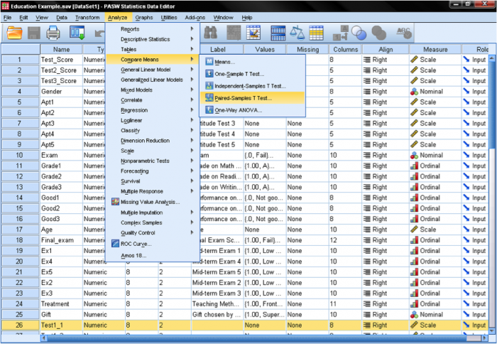
We need to specify the paired variable in the dialog box for the dependent samples t-test. We need to inform SPSS what is the before and after measurement. SPSS automatically assumes that the second dimension of the pairing is the case number, i.e. that case number 1 is a pair of measurements between variable 1 and 2.
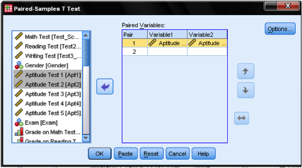
Although we could specify multiple dependent samples t-test that are executed at the same time, our example only looks at the first and the second aptitude test. Thus we drag & drop ‘Aptitude Test 1 ‘ into the cell of pair 1 and variable 1, and ‘Aptitude Test 2’ into the cell pair 1 and variable 2. The Options… button allows to define the width of the control interval and how missing values are managed. We leave all settings as they are.
Paired T Test Calculator (Dependent T test)
Enter sample data

Reporting results in APA style
Paired t-test online, what is a paired t-test, how to use the paired t-test calculator, calculators.
A comprehensive comparison of goodness-of-fit tests for logistic regression models
- Original Paper
- Published: 30 August 2024
- Volume 34 , article number 175 , ( 2024 )
Cite this article

- Huiling Liu 1 ,
- Xinmin Li 2 ,
- Feifei Chen 3 ,
- Wolfgang Härdle 4 , 5 , 6 &
- Hua Liang 7
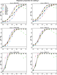
We introduce a projection-based test for assessing logistic regression models using the empirical residual marked empirical process and suggest a model-based bootstrap procedure to calculate critical values. We comprehensively compare this test and Stute and Zhu’s test with several commonly used goodness-of-fit (GoF) tests: the Hosmer–Lemeshow test, modified Hosmer–Lemeshow test, Osius–Rojek test, and Stukel test for logistic regression models in terms of type I error control and power performance in small ( \(n=50\) ), moderate ( \(n=100\) ), and large ( \(n=500\) ) sample sizes. We assess the power performance for two commonly encountered situations: nonlinear and interaction departures from the null hypothesis. All tests except the modified Hosmer–Lemeshow test and Osius–Rojek test have the correct size in all sample sizes. The power performance of the projection based test consistently outperforms its competitors. We apply these tests to analyze an AIDS dataset and a cancer dataset. For the former, all tests except the projection-based test do not reject a simple linear function in the logit, which has been illustrated to be deficient in the literature. For the latter dataset, the Hosmer–Lemeshow test, modified Hosmer–Lemeshow test, and Osius–Rojek test fail to detect the quadratic form in the logit, which was detected by the Stukel test, Stute and Zhu’s test, and the projection-based test.
This is a preview of subscription content, log in via an institution to check access.
Access this article
Subscribe and save.
- Get 10 units per month
- Download Article/Chapter or eBook
- 1 Unit = 1 Article or 1 Chapter
- Cancel anytime
Price includes VAT (Russian Federation)
Instant access to the full article PDF.
Rent this article via DeepDyve
Institutional subscriptions
A generalized Hosmer–Lemeshow goodness-of-fit test for a family of generalized linear models

Fifty Years with the Cox Proportional Hazards Regression Model

CPMCGLM: an R package for p -value adjustment when looking for an optimal transformation of a single explanatory variable in generalized linear models
Explore related subjects.
- Artificial Intelligence
Data availibility
No datasets were generated or analysed during the current study.
Chen, K., Hu, I., Ying, Z.: Strong consistency of maximum quasi-likelihood estimators in generalized linear models with fixed and adaptive designs. Ann. Stat. 27 (4), 1155–1163 (1999)
Article MathSciNet Google Scholar
Dardis, C.: LogisticDx: diagnostic tests and plots for logistic regression models. R package version 0.3 (2022)
Dikta, G., Kvesic, M., Schmidt, C.: Bootstrap approximations in model checks for binary data. J. Am. Stat. Assoc. 101 , 521–530 (2006)
Ekanem, I.A., Parkin, D.M.: Five year cancer incidence in Calabar, Nigeria (2009–2013). Cancer Epidemiol. 42 , 167–172 (2016)
Article Google Scholar
Escanciano, J.C.: A consistent diagnostic test for regression models using projections. Economet. Theor. 22 , 1030–1051 (2006)
Härdle, W., Mammen, E., Müller, M.: Testing parametric versus semiparametric modeling in generalized linear models. J. Am. Stat. Assoc. 93 , 1461–1474 (1998)
MathSciNet Google Scholar
Harrell, F.E.: rms: Regression modeling strategies. R package version 6.3-0 (2022)
Hosmer, D.W., Hjort, N.L.: Goodness-of-fit processes for logistic regression: simulation results. Stat. Med. 21 (18), 2723–2738 (2002)
Hosmer, D.W., Lemesbow, S.: Goodness of fit tests for the multiple logistic regression model. Commun Stat Theory Methods 9 , 1043–1069 (1980)
Hosmer, D.W., Hosmer, T., Le Cessie, S., Lemeshow, S.: A comparison of goodness-of-fit tests for the logistic regression model. Stat. Med. 16 (9), 965–980 (1997)
Hosmer, D., Lemeshow, S., Sturdivant, R.: Applied Logistic Regression. Wiley Series in Probability and Statistics, Wiley, New York (2013)
Book Google Scholar
Jones, L.K.: On a conjecture of Huber concerning the convergence of projection pursuit regression. Ann. Stat. 15 , 880–882 (1987)
Kohl, M.: MKmisc: miscellaneous functions from M. Kohl. R package version, vol. 1, p. 8 (2021)
Kosorok, M.R.: Introduction to Empirical Processes and Semiparametric Inference, vol. 61. Springer, New York (2008)
Lee, S.-M., Tran, P.-L., Li, C.-S.: Goodness-of-fit tests for a logistic regression model with missing covariates. Stat. Methods Med. Res. 31 , 1031–1050 (2022)
Lindsey, J.K.: Applying Generalized Linear Models. Springer, Berlin (2000)
McCullagh, P., Nelder, J.A.: Generalized Linear Models, vol. 37. Chapman and Hall (1989)
Nelder, J.A., Wedderburn, R.W.M.: Generalized linear models. J. R. Stat. Soc. Ser. A 135 , 370–384 (1972)
Oguntunde, P.E., Adejumo, A.O., Okagbue, H.I.: Breast cancer patients in Nigeria: data exploration approach. Data Brief 15 , 47 (2017)
Osius, G., Rojek, D.: Normal goodness-of-fit tests for multinomial models with large degrees of freedom. J. Am. Stat. Assoc. 87 (420), 1145–1152 (1992)
Rady, E.-H.A., Abonazel, M.R., Metawe’e, M.H.: A comparison study of goodness of fit tests of logistic regression in R: simulation and application to breast cancer data. Appl. Math. Sci. 7 , 50–59 (2021)
Google Scholar
Stukel, T.A.: Generalized logistic models. J. Am. Stat. Assoc. 83 (402), 426–431 (1988)
Stute, W., Zhu, L.-X.: Model checks for generalized linear models. Scand. J. Stat. Theory Appl. 29 , 535–545 (2002)
van der Vaart, A.W., Wellner, J.A.: Weak Convergence and Empirical Processes. Springer (1996)
van Heel, M., Dikta, G., Braekers, R.: Bootstrap based goodness-of-fit tests for binary multivariate regression models. J. Korean Stat. Soc. 51 (1), 308–335 (2022)
Yin, C., Zhao, L., Wei, C.: Asymptotic normality and strong consistency of maximum quasi-likelihood estimates in generalized linear models. Sci. China Ser. A Math. 49 , 145–157 (2006)
Download references
Acknowledgements
Li’s research was partially supported by NNSFC grant 11871294. Härdle gratefully acknowledges support through the European Cooperation in Science & Technology COST Action grant CA19130 - Fintech and Artificial Intelligence in Finance - Towards a transparent financial industry; the project “IDA Institute of Digital Assets”, CF166/15.11.2022, contract number CN760046/ 23.05.2024 financed under the Romanias National Recovery and Resilience Plan, Apel nr. PNRR-III-C9-2022-I8; and the Marie Skłodowska-Curie Actions under the European Union’s Horizon Europe research and innovation program for the Industrial Doctoral Network on Digital Finance, acronym DIGITAL, Project No. 101119635
Author information
Authors and affiliations.
Department of Statistics, South China University of Technology, Guangzhou, China
Huiling Liu
School of Mathematics and Statistics, Qingdao University, Shandong, 266071, China
Center for Statistics and Data Science, Beijing Normal University, Zhuhai, 519087, China
Feifei Chen
BRC Blockchain Research Center, Humboldt-Universität zu Berlin, 10178, Berlin, Germany
Wolfgang Härdle
Dept Information Management and Finance, National Yang Ming Chiao Tung U, Hsinchu, Taiwan
IDA Institute Digital Assets, Bucharest University of Economic Studies, Bucharest, Romania
Department of Statistics, George Washington University, Washington, DC, 20052, USA
You can also search for this author in PubMed Google Scholar
Contributions
LHL, LXM and LH wrote the main manuscript text, LHL and CFF program, HW commented on the methodological section. All authors reviewed the manuscript.
Corresponding author
Correspondence to Hua Liang .
Ethics declarations
Competing interests.
The authors declare no competing interests.
Additional information
Publisher's note.
Springer Nature remains neutral with regard to jurisdictional claims in published maps and institutional affiliations.
Rights and permissions
Springer Nature or its licensor (e.g. a society or other partner) holds exclusive rights to this article under a publishing agreement with the author(s) or other rightsholder(s); author self-archiving of the accepted manuscript version of this article is solely governed by the terms of such publishing agreement and applicable law.
Reprints and permissions
About this article
Liu, H., Li, X., Chen, F. et al. A comprehensive comparison of goodness-of-fit tests for logistic regression models. Stat Comput 34 , 175 (2024). https://doi.org/10.1007/s11222-024-10487-5
Download citation
Received : 02 December 2023
Accepted : 19 August 2024
Published : 30 August 2024
DOI : https://doi.org/10.1007/s11222-024-10487-5
Share this article
Anyone you share the following link with will be able to read this content:
Sorry, a shareable link is not currently available for this article.
Provided by the Springer Nature SharedIt content-sharing initiative
- Consistent test
- Model based bootstrap (MBB)
- Residual marked empirical process (RMEP)
- Find a journal
- Publish with us
- Track your research
- Open access
- Published: 31 August 2024
Accelerometer-derived movement features as predictive biomarkers for muscle atrophy in neurocritical care: a prospective cohort study
- Moritz L. Schmidbauer 1 na1 ,
- Timon Putz 1 na1 ,
- Leon Gehri 1 ,
- Luka Ratkovic 1 ,
- Andreas Maskos 1 ,
- Julia Zibold 1 ,
- Johanna Bauchmüller 1 ,
- Sophie Imhof 1 ,
- Thomas Weig 2 ,
- Max Wuehr 1 , 3 na1 &
- Konstantinos Dimitriadis 1 na1
Critical Care volume 28 , Article number: 288 ( 2024 ) Cite this article
Metrics details
Physical inactivity and subsequent muscle atrophy are highly prevalent in neurocritical care and are recognized as key mechanisms underlying intensive care unit acquired weakness (ICUAW). The lack of quantifiable biomarkers for inactivity complicates the assessment of its relative importance compared to other conditions under the syndromic diagnosis of ICUAW. We hypothesize that active movement, as opposed to passive movement without active patient participation, can serve as a valid proxy for activity and may help predict muscle atrophy. To test this hypothesis, we utilized non-invasive, body-fixed accelerometers to compute measures of active movement and subsequently developed a machine learning model to predict muscle atrophy.
This study was conducted as a single-center, prospective, observational cohort study as part of the MINCE registry (metabolism and nutrition in neurointensive care, DRKS-ID: DRKS00031472). Atrophy of rectus femoris muscle (RFM) relative to baseline (day 0) was evaluated at days 3, 7 and 10 after intensive care unit (ICU) admission and served as the dependent variable in a generalized linear mixed model with Least Absolute Shrinkage and Selection Operator regularization and nested-cross validation.
Out of 407 patients screened, 53 patients (age: 59.2 years (SD 15.9), 31 (58.5%) male) with a total of 91 available accelerometer datasets were enrolled. RFM thickness changed − 19.5% (SD 12.0) by day 10. Out of 12 demographic, clinical, nutritional and accelerometer-derived variables, baseline RFM muscle mass (beta − 5.1, 95% CI − 7.9 to − 3.8) and proportion of active movement (% activity) (beta 1.6, 95% CI 0.1 to 4.9) were selected as significant predictors of muscle atrophy. Including movement features into the prediction model substantially improved performance on an unseen test data set (including movement features: R 2 = 79%; excluding movement features: R 2 = 55%).
Active movement, as measured with thigh-fixed accelerometers, is a key risk factor for muscle atrophy in neurocritical care patients. Quantifiable biomarkers reflecting the level of activity can support more precise phenotyping of ICUAW and may direct tailored interventions to support activity in the ICU. Studies addressing the external validity of these findings beyond the neurointensive care unit are warranted.
Trial registration
DRKS00031472, retrospectively registered on 13.03.2023.
Intensive care unit acquired weakness (ICUAW) describes a neuromuscular dysfunction secondary to critical illness and its treatment with consecutive generalized weakness. Data on prevalence for ICUAW show considerable variation due to diverse patient demographics and heterogenous methodology. However, with a systematic review pinpointing the median prevalence at 43% [ 1 ], its ubiquity in critical care is evident. Moreover, the impact resulting from ICUAW is profound and long-lasting, with patient outcomes significantly compromised for up to five years after discharge [ 2 , 3 , 4 , 5 , 6 ]. Therefore, ICUAW is acknowledged as a key component of post intensive care syndrome (PICS), highlighting its importance in the continuum of long-term recovery following critical care [ 7 , 8 ].
ICUAW needs to be recognized as a clinical syndrome, rather than a specific disease entity. As such, it exhibits great heterogeneity and partially overlapping pathologies, which has diluted research findings and made the identification of treatable targets challenging in the past [ 9 , 10 , 11 , 12 ]. Relevant and common entities include critical illness myopathy (CIM), critical illness polyneuropathy (CIP) as well as critical illness polyneuromyopathy (CIPNM) as an overlap syndrome [ 9 , 11 , 12 ]. Electrophysiological methods including nerve conduction studies (NCS), electromyography and direct muscle stimulation have been successfully used to establish biomarkers for CIM, CIP and CIPMN [ 9 , 13 , 14 ]. Muscle atrophy due to mechanical unloading is also being recognized as a critical component of ICUAW. However, measurable biomarkers to assess the extent of inactivity of muscles are lacking.
In this regard, it is important to note that activity arises from active movement, as opposed to passive movement during mobilization without active patient participation. Hence, we postulate that establishing a proxy for activity can be achieved by applying non-invasive, body-fixed accelerometers to the lower extremities of critically ill patients while prospectively excluding episodes with passive mobilization such as intrahospital transports, physiotherapy and patient positioning. By introducing these biomarkers as continuous measures of active movement and incorporating these variables into a machine learning model, we aimed to predict rectus femoris muscle atrophy, as measured by ultrasound up to day 10 of intensive care unit (ICU) treatment. Based on the hypothesis that neurocritical care patients exhibit a higher prevalence of inactivity due to disorders of consciousness and motor deficits, we specifically included patients with acute brain injury in this trial.
Study design, setting and clinical management
This study was designed as a single-center, prospective, observational cohort study as part of the MINCE registry (metabolism and nutrition in neurointensive care, DRKS-ID: DRKS00031472, retrospectively registered on 13.03.2023) at a tertiary academic center (LMU University Hospital, Munich, Germany). Reporting follows the Strengthening the Reporting of Observational Studies in Epidemiology (STROBE) reporting guidelines. This study was approved by the local ethics committee (LMU Munich, project number 22-0173, 11.04.2022). Written consent was obtained from all participants or their next of kin. The study recruited from April 2022 to March 2024 and included patients within 48 h after ICU admission with age ≥ 18 years, neurologic disease as admitting diagnosis, and expected ICU length of stay ≥ 10 days. Patients with pre-existing neuromuscular disease, renal replacement therapy, pregnancy, pre-existing neoplastic disease, recent hospitalization (hospital stays longer than three days in the last three months, ICU treatment within the last three months), pre-existing confinement to bed, and pre-existing frailty (Clinical Frailty Scale > 3) were excluded.
Patients were mobilized at the treating physicians’ discretion. If indicated, patients received physiotherapy for 20–40 min/day on six days of the week and were repositioned and transferred from bed to chair regularly by the nursing staff. Nutritional therapy was conducted according to the European Society of Parenteral and Enteral Nutrition (ESPEN) guidelines, with caloric and protein targets of 25 kcal/kg/day and 1.3 g/kg/day, respectively [ 15 ]. As a reference, body weight as measured with bed scales was used for non-obese patients, and ideal body weight was used for patients with a body mass index (BMI) > 30 kg/m 2 [ 15 ]. During the acute phase of illness (days 1–3), hypocaloric nutrition (70% of energy expenditure (EE)) was aimed for. From day 4 on, isocaloric (100% of EE) nutrition was implemented.
Data collection
Clinical data prospectively collected on the ICU included age, sex, body mass index (BMI), admission diagnosis, cumulative protein and calorie deficit, duration of mechanical ventilation, ICU length of stay (LOS), daily Sepsis-related Organ Failure Assessment score (SOFA) and SOFA without Glasgow Coma Scale (GCS) score (mSOFA), Acute Physiology and Chronic Health Evaluation (APACHE II) score on ICU admission, Nutrition Risk in Critically ill score (NUTRIC) on admission, premorbid modified Rankin Scale (pmRS) and Glasgow Outcome Scale Extended (GOSE) at ICU discharge.
Ultrasound of the upper thigh (rectus femoris muscle, RFM) and temporalis muscle (TM) was performed bilaterally using a 20 MHz linear probe (MyLabOmega, Esaote, Genoa, Italy) upon admission, and on days 3, 7 and 10. As previously described [ 16 , 17 ], the site of measurement for RFM was marked in the lower third of the connecting line between the anterior superior iliac spine and the upper edge of the patella with a permanent marker to ensure reproducibility between measurements (Supplementary Fig. 1 ). Measurements were conducted according to a local protocol that emphasized minimal compression during RFM sonography and called for individual adjustments of depth and gain to optimally visualize the surface of the femur and to delineate fascial borders, respectively. Measurement of TM followed the protocol as described by Maskos et al. [ 17 ] Three repeated measurements were performed by one of six raters (TP, LG, LR, AM, JB, SI), using the built-in software of the ultrasound machine to measure muscle thickness. The mean value of the repeated measurements was used for further analysis. Reliability of repeated ultrasound measurements is reported in Supplementary Table 1 .
Tri-axial accelerometers (range ± 16 g; sampling rate 12.5 Hz; Axivity Ltd., Newcastle upon Tyne, UK) were attached within 48 h of admission to both upper thighs with transparent adhesive tape. Skin inspections and minor adjustments to the sensor placement were performed every third day to prevent any pressure damage. To exclude any passive movement not contributing to the patient’s activity, episodes with physiotherapy, intrahospital transports, or repositioning by nursing staff were prospectively documented and excluded from the recorded data. The sensor data was extracted and analyzed by an author (MW) not involved in the patients’ clinical management and blinded for the ultrasound measurements.
As a positive control, accelerometers were attached to healthy individuals (n = 3). Static placement of sensors served as a negative control (Supplementary Table 2 ).
Accelerometer data processing
OmGUI version 1.0.0.11 software was used to download the raw acceleration data from the devices. MATLAB (Mathworks Inc., Natick, USA, release R2022a, version 9.12.0) was used for data processing. Periods of active movement were identified following a previously established procedure that has been already used for activity recognition in ICU settings [ 18 , 19 ]. Accordingly, recorded time series from each axial component (x, y, z) were first down-sampled to 10 Hz and subsequently high-pass filtered (4th order Butterworth filter, cutoff frequency at 0.2 Hz) to remove baseline offset and low-frequency effects reflecting static postural orientation. Filtered time series were segmented into non-overlapping 5 s windows for subsequent motion feature extraction. Signal magnitude area (SMA) was then computed for every window [ 19 ] to identify activity bouts (AB) using a defined threshold of SMA ≥ 0.135 g [ 18 ]. Across all identified AB, the mean intensity (AB-intensity) and duration (AB-duration) as well as the variability (standard deviation, SD) of these features were calculated. The distribution of motion features across ABs is log-normal, which required estimating mean and SD via a maximum likelihood technique [ 20 ]. The overall movement intensity, the proportion of active movement (%active) and ABs per hour were calculated based on the entire duration of the recording (Fig. 1 ).

Accelerometer-derived features. Body motion was monitored using tri-axial accelerometers bilaterally attached to the upper thigh (1). Raw triaxial accelerometer recordings were first offset eliminated, and the time series were segmented into non-overlapping 5 s windows. The signal magnitude area was computed for every window (2). Bouts of dynamic activity were identified based on the threshold ≥ 0.135 g (3) and a set of motion features was computed for every bout of activity (4). Finally, the average and distribution of motion features across all bouts of activity were computed (5). acc = acceleration
Predictive modeling and statistical analysis
As the dataset includes multiple observations (both legs) per patient and exhibits linearity as evaluated by exploratory data analysis, a generalized linear mixed model (GLMM) to account for intra-patient correlation by using individual patients as a random effect was chosen. Given the numerous independent variables of interest, including demographic, clinical, and activity-related features, a rigorous approach to model selection and validation to prevent overfitting was required. Therefore, we employed regularization with Least Absolute Shrinkage and Selection Operator (LASSO), which penalizes the GLMM model via L1-norm and in effect shrinks the weight of non-contributing features to zero.
First, multicollinearity among predictors was mitigated by excluding variables with a variance inflation factor (VIF) exceeding 5 (removing AB per hour and SOFA) [ 21 ]. Next, standardization (z-score normalization) of the remaining prediction variables (age, sex, baseline RFM muscle mass, mSOFA, calorie deficit, protein deficit, overall intensity, %active, AB-intensity log-mean , AB-duration log-mean , AB-intensity log-SD , AB-duration log-SD ) was performed to ensure equal weights and comparable units. To allow testing on unseen data, a stratified split was executed to divide the data into training (80%) and test (20%) sets. The training set was further used for optimizing the hyperparameter of GLMM-LASSO using a machine learning approach with nested cross-validation (Fig. 2 ) [ 22 ]. Model performance was evaluated on the test set using mean squared error, root mean squared error, mean absolute error, R-squared (squared correlation method, R2) and a plot depicting actual versus predicted values.

Nested-cross validation of a regularized GLMM model . After standardization and a stratified 80/20 split, the training data set was partitioned into 4 folds (outer loop). Within each outer fold, an inner loop of 2 folds was used for hyperparameter tuning. The hyperparameter (lambda) that minimized the mean squared error in the inner loop was selected. The model with this optimal lambda was then evaluated on the validation fold of the outer loop. This process was repeated for all 4 outer folds, resulting in an optimal lambda for each fold. The final model was chosen using the average of the optimal lambdas from all outer folds. Finally, the performance of this final model was assessed using the unseen test set. GLMM = generalized mixed effects model; lasso = least absolute shrinkage and selection operator
To illustrate the level of uncertainty of the model coefficients, bootstrapping with 10,000 resamples was performed to estimate the bias-corrected and accelerated (BCa) confidence intervals for the model coefficients.
Additionally, and to test the relevance of leg movement on TM as a muscle group unaffected by thigh movement, we used a linear regression model for the prediction of TM atrophy at day 10 including all demographic, clinical and nutritional variables as well as %active as independent variables. To compare %active between healthy individuals and the neurointensive care unit (NICU) cohort, a two-tailed t-test was performed. Further, we identified patients with unilateral upper motor neuron damage and corresponding motor deficits to investigate the contribution of upper motor neuron lesion on muscle atrophy. To compare the magnitude of muscle atrophy and to account for within-subject correlation, we used Generalized Estimating Equations (GEE) with post hoc pairwise comparisons and Bonferroni adjustment.
Summary statistics for continuous variables are presented as means with standard deviation (SD) for normally distributed data and as medians with interquartile ranges (IQR) for non-normally distributed data, with normality assessed using Quantile–Quantile plots and Shapiro–Wilk test. Categorical variables are summarized as frequencies and percentages.
All analyses were performed using R (2023.06.1 + 524) using ‘stats’, ‘psych’, ‘ggplot2’, ‘dplyr’, ‘lme4’, ‘nlme’, ‘geepack’, ‘multcomp’, ‘emmeans’, ‘MASS’, ‘svglite’ ‘glmmLasso’,‘caret’ and ‘boot’, packages. ChatGPT (version 4) was used for error handling, repetitive programming, and overall optimization of code in R.
Patient characteristics
Out of 407 patients screened, 53 with a total of 91 available accelerometer datasets were enrolled in this study (Fig. 3 ). Clinical baseline characteristics are presented in Table 1 . Of all patients included in the analysis, mean age was 59.2 years (SD 15.9) and 31 (58.5%) were male. Cerebrovascular diseases were the most frequent ICU admission diagnoses (86.8%, 46/53). Mean ICU length of stay was 17.0 days (IQR 8.0), while the mean duration of mechanical ventilation was 15.6 days (SD 9.2). During the observation period, patients met 62.6% (SD 18.4) of the caloric goals and 57.9% (SD 21.6) of protein goals according to the ESPEN guidelines.

Screening and study inclusion. ICU = Intensive Care Unit;
Active movement and muscle atrophy during ICU treatment
Muscular atrophy as measured with ultrasound was more pronounced in RFM compared to TM (-19.5% (SD 12.0) versus -15.3% (SD 11.1) at day 10) (Fig. 4 A). Active movement of NICU patients as indicated by proportion of active movement (%active) over time is infrequent, particular at early stages of the ICU stay. While mean %active stays low over the entire time, some patients exhibit higher activity starting around day 3. (Fig. 4 B). Compared to healthy individuals, NICU patients demonstrate a significant reduction in active movement (%active: healthy individuals 13.3 (SD 0.8) vs. NICU patients 0.84 (SD 1.08), p < 0.001) (Supplementary Tables 2 and 4 ). No adverse events were observed in association with the placement of accelerometers in the ICU setting (Supplementary Table 3 ).

Active movement and muscle atrophy during ICU treatment. Muscle atrophy at days 3, 5 7 and 10 relative to day 0 for RFM and TM ( A ). Proportion of active movement (%active) over time ( B ). ICU = Intensive Care Unit;
Predictive models for muscle atrophy
The machine learning model based on a total of 12 demographic, clinical, nutritional and accelerometer-derived variables selected baseline RFM muscle mass (beta − 5.1, 95% confidence interval (95% CI) − 7.9 to − 3.8) and %active (beta 1.6, 95% CI 0.1 to 4.9) to explain 79% (R 2 = 79%) of the occurring variance in muscle wasting in an unseen test data set (Fig. 5 , A and B). Thus, for every standard deviation increase in baseline RFM (2.6 mm), RFM thickness at day 10 is estimated to decrease by another 5.1 percentage points (49.5% relative change). In contrast, a standard unit increase in %active (1.1%) is projected to result in 1.6 percentage points less RFM atrophy at day 10 (relative change 15.5%). Ignoring movement features as predictors for RFM muscle atrophy results in substantially worse model performance (R 2 = 55%) (Fig. 5 C, Supplementary Table 6 ). RFM atrophy was not significantly different between immobile limbs with upper motor neuron lesions (UMNL) and immobile limbs without UMNL. However, muscle atrophy was markedly decreased in limbs with active movement (Supplementary Fig. 2 ). Thigh-fixed accelerometer data did not contribute significantly to a model predicting TM atrophy (Supplementary Table 5 ).

Prediction of MRF muscle atrophy with and without movement features. Standardized coefficients and 95% confidence intervals (asterisks indicate significant predictors) of the regularized regression models with (model movement+ , A ) and without movement features (model movement− , C ). Out of all demographic (age, sex), clinical (baseline RFM muscle mass, mSOFA), nutritional (calorie deficit, protein deficit) and movement variables (intensity, %active, AB-intensity log-mean , AB-duration log-mean , AB-intensity log-SD , AB-duration log-SD ), the depicted 10/12 independent variables for model model movement+ and 4/6 independent variables for model movement− were selected for the final models, respectively. Significant predictors in model movement+ included baseline RFM muscle mass (beta − 5.1, 95% confidence interval (95% CI) − 7.9 to − 3.8) and %active (beta 1.6, 95% CI 0.1 to 4.9). For model movement- , only baseline RFM muscle was found as a statistically significant predictor (beta − 4.6, 95% CI − 7.6 to − 3.9). Scatter plots with regression line of predicted versus actual muscle wasting (grey dots: training data; black dots: unseen test data) for model movement+ ( B ) and model movement- ( D ), respectively (R 2 : 0.79 vs. 0.55, RMSE: vs. 8.4 vs. 10.7 mm; MAE: 6.2 vs. 8.0 mm). mSOFA = SOFA without GCS;
In this prospective cohort study, we used thigh-fixed accelerometers to establish movement features as predictive biomarkers for muscle atrophy in neurocritical care patients. Proportion of active movement (%active) demonstrated a significant protective effect against muscle wasting and improved the precision of muscle atrophy prediction in an unseen test data set. To the best of our knowledge, this is the first quantifiable and validated measure that provides information on the relative importance of inactivity for muscle atrophy in critically ill patients.
It is crucial to distinguish between immobility and inactivity, especially within the ICU context, as inactivity can occur despite mobilization efforts due to a lack of active patient participation (passive movement). To address this, we excluded periods such as physiotherapy, intrahospital transports, and patient positioning, from our analysis. Therefore, we consider the movement features as surrogates for activity rather than measures of mobility. Importantly, and as a limitation of this approach, movement sensors are unable to capture any muscle activity without movement via isometric contractions (active immobility).
The relevance of inactivity, as compared to immobility, as the variable of interest in this context is further exemplified by clinical trials on electrical muscle stimulation (EMS) and interventions focusing on early (passive) mobilization. The current evidence highlights the efficacy of EMS [ 23 , 24 ], whereas mobilization trials demonstrated limited efficacy and raised safety concerns [ 25 , 26 , 27 , 28 , 29 , 30 , 31 ]. While the latter often involve passive mobilization without genuine patient activity, EMS generates muscle activity without requiring mobility. Considering the data, a reasonable strategy to prevent muscle atrophy in critically ill patients may involve first measuring the extent of active movement with accelerometers to identify those at risk, and subsequently promoting activity (with or without mobilization) based on the patient's stability.
The pathophysiology of mechanical unloading leading to atrophy has so far only been systematically studied and quantified outside the ICU. Studies with cast immobilization of the lower extremity for two weeks in healthy adults and examination of astronauts after 8 days of space flight revealed a 5% and 6% decrease in quadriceps muscle mass, respectively [ 32 , 33 ]. A recent meta-analysis analyzing the general ICU population estimated muscle atrophy to be around 16% at day 10 for RFM [ 34 ]. In comparison, our data demonstrate a more pronounced rate of RFM atrophy, showing a 19.5% decrease by day 10. While additional factors such as CIP, CIM, and CIPNM certainly contribute to the higher rate of atrophy in ICU patients, the residual activity in cast immobilization (via isometric contractions) and during space flight (via active movement with reduced muscle activity) may also account for the observed differences.
Given that no or passive movement was described in more than 70% of patients in the first 48 h, and still more than 40% after two weeks, in the TEAM trial [ 26 ], it is plausible to assume that inactivity also significantly contributes to ICUAW in the general ICU population. Yet, as disorders of consciousness and focal-neurological deficits are major barriers to mobilization and activity [ 26 ], this might be even more relevant for neurointensive care patients. Although our accelerometer data are not directly comparable to the ICU mobility scale used in the TEAM trial, it indicates extremely infrequent periods of active movement for most patients over a 10-day observation period, reaching only 6% (0.84/13.3) of the activity level of healthy individuals. These numbers are parallelled by data from González-Seguel et al., who found mechanically ventilated patients to be inactive during the ICU stay in over 96% of the time [ 35 ]. This, coupled with the prominence of movement features as predictors of muscle atrophy in our prospective cohort, further strengthens the significance of inactivity in (neuro-) critical care. Other studies within the ICU have investigated accelerometry primarily in the context of sleep, circadian rhythm, and sedation levels. However, these studies exhibit limitations, such as narrow observation periods and the absence of well-defined thresholds for activity measurement [ 36 , 37 , 38 , 39 ].
Accelerometer-derived data have also been validated as biomarkers for muscle atrophy outside the ICU setting. In a study with almost 500 elderly participants, Sanchez-Sanchez et al. investigated the association of physical activity as measured with hip-worn accelerometers and sarcopenia. Here, higher physical activity correlated with better performance in sarcopenia-related scores [ 40 ]. Similarly, Foong et al. showed a positive association of accelerometer-derived physical activity with muscle mass and muscle strength [ 41 ].
The exercise stimulus, as the ultimate determinant for activity, can be delineated into two primary variables: volume and intensity. In exercise physiology, the volume of exercise is traditionally quantified by the number of repetitions performed, while intensity is commonly measured by the force exerted during exercise [ 42 ]. In our ICU cohort, we utilized proportion of active movement (%active) and AB-duration log-mean as proxies for exercise volume. For critically ill patients, the force generated cannot be measured pragmatically. We therefore introduced movement intensity (resultant acceleration magnitude) as a surrogate of exercise intensity. The LASSO regularization used to address the high number and potential co-linearity of parameters revealed %active as an approximation of exercise volume as a relevant predictor, while surrogates of intensity were not selected. Thus, intensity may either be irrelevant considering the uniform force generated by patients moving against gravity and not against resistance, or movement intensity is not a valid biomarker of the exercise intensity.
Besides proportion of active movement, baseline muscle mass was predictive of muscle atrophy. This finding is in line with studies in healthy participants. Here, higher age with lower baseline muscle mass showed significantly less pronounced atrophy. However, older participants with lower baseline muscle mass suffered from greater loss of muscle strength after immobilization [ 43 , 44 , 45 ]. Furthermore, variations in atrophy can be observed across muscle and fiber types. Anti-gravity muscles with high proportions of slow type 1 fibers, such as RFM, seem to exhibit a selective vulnerability [ 45 ], which is in line with our data demonstrating pronounced atrophy of RFM over TM.
The strengths of our study include the selection of a neurointensive care population devoid of frailty, specifically targeting individuals at high risk of muscle atrophy without pre-existing muscle wasting. However, the study's focus on neurocritical care may limit its generalizability and further research is needed to confirm the applicability of our results to more diverse patient populations. The extent of neurogenic atrophy mediated via various damage to the lower motor neuron was not explicitly measured in our study but can be assumed to be minimal given the demographics of our cohort. As that general ICU cohorts also experience lower motor neuron lesions due to critical illness or its treatments, this confounder is likely to be similar across groups. For UMNL, we do not expect neurogenic atrophy, as it does not result in direct muscle denervation. Supporting this pathophysiological hypothesis, we could not observe any difference in the extent of muscle atrophy between immobile limbs with upper motor neuron lesions (UMNL) and immobile limbs without UMNL. However, muscle atrophy was markedly decreased in limbs with active movement, suggesting no role for UMNL as a mediator for atrophy. We ensured high data quality by filtering out passive mobilization and prospectively collecting clinical data. Furthermore, our analysis is underpinned by a strong statistical framework leveraging machine learning to identify the most important predictors and using unseen data to validate these findings. Further limitations of our study are primarily rooted in the fact that muscle morphology does not necessarily equate to function. We used muscle ultrasound, a widely adopted and validated surrogate for ICUAW [ 34 , 46 , 47 ], instead of the Medical Research Council Sum Score (MRC-SS), as the latter is often deemed infeasible in the general ICU cohort, and even more so in neurocritical care. Additionally, we decided against including measures of the upper extremities because muscle volume is challenging to determine via ultrasound due to variability in muscle thickness relative to positioning, difficult anatomical landmarks, and less pronounced atrophy compared to the lower extremities. Instead, we focused on the RFM as the established sonographic gold standard, along with the TM as a muscle group unrelated to the movement captured by the accelerometers.
Active movement, as a surrogate of muscle activity, can be quantified using non-invasive, thigh-fixed accelerometers and adds value for the prediction of muscle atrophy in neurocritical care patients. Establishing movement-derived biomarkers enables better phenotyping of ICUAW, thereby providing a foundation for tailored interventions and should be included as covariates in trials on ICUAW in the future. Studies addressing the external validity of these findings beyond the neurointensive care unit are warranted.
Availability of data and materials
The datasets used and/or analyzed during the current study are available from the corresponding author on reasonable request. Matlab code for analyzing motion features is available at https://github.com/DSGZ-MotionLab/ICU_motion_analysis/ .
Abbreviations
Activity bout
Acute physiology and chronic health evaluation II
Bias-corrected and accelerated
Body mass index
Confidence interval
Critical illness myopathy
Critical illness polyneuropathy
Critical illness polyneuromyopathy
Energy expenditure
Electrical muscle stimulation
European Society of Parenteral and Enteral Nutrition
Glasgow Coma Scale
Generalized Estimating Equations
Generalized linear mixed model
Glasgow Outcome Scale—Extended
High/low pass filter
Intensive care unit
Intensive care unit acquired weakness
Least Absolute Shrinkage and Selection Operator
Length of stay
Metabolism and nutrition in neurointensive care
Medical Research Council Sum Score
Modified SOFA
Nerve conduction studies
Neurointensive care unit
Nutrition risk in the critically ill
Post intensive care syndrome
Premorbid modified Rankin scale
Quantile–Quantile
Rectus femoris muscle
Signal magnitude area
Sequential organ failure assessment
Temporalis muscle
Upper motor neuron lesion
Fan E, Cheek F, Chlan L, Gosselink R, Hart N, Herridge MS, et al. An official American Thoracic Society Clinical Practice guideline: the diagnosis of intensive care unit–acquired weakness in adults. Am J Respir Crit Care Med. 2014;190:1437–46.
Article PubMed Google Scholar
Van Aerde N, Meersseman P, Debaveye Y, Wilmer A, Gunst J, Casaer MP, et al. Five-year impact of ICU-acquired neuromuscular complications: a prospective, observational study. Intensive Care Med. 2020;46:1184–93.
Kelmenson DA, Held N, Allen RR, Quan D, Burnham EL, Clark BJ, et al. Outcomes of ICU patients with a discharge diagnosis of critical illness polyneuromyopathy: a propensity-matched analysis. Crit Care Med. 2017;45:2055–60.
Article PubMed PubMed Central Google Scholar
Saccheri C, Morawiec E, Delemazure J, Mayaux J, Dubé B-P, Similowski T, et al. ICU-acquired weakness, diaphragm dysfunction and long-term outcomes of critically ill patients. Ann Intensive Care. 2020;10:1. https://doi.org/10.1186/s13613-019-0618-4 .
De Jonghe B, Sharshar T, Lefaucheur J-P, Authier F-J, Durand-Zaleski I, Boussarsar M, et al. Paresis acquired in the intensive care unit: a prospective multicenter study. JAMA. 2002;288:2859–67.
Hermans G, Van Mechelen H, Bruyninckx F, Vanhullebusch T, Clerckx B, Meersseman P, et al. Predictive value for weakness and 1-year mortality of screening electrophysiology tests in the ICU. Intensive Care Med. 2015;41:2138–48.
Needham DM, Davidson J, Cohen H, Hopkins RO, Weinert C, Wunsch H, et al. Improving long-term outcomes after discharge from intensive care unit. Crit Care Med. 2012;40:502–9.
Hermans G, Van den Berghe G. Clinical review: intensive care unit acquired weakness. Crit Care. 2015;19:274.
Vanhorebeek I, Latronico N, Van den Berghe G. ICU-acquired weakness. Intensive Care Med. 2020;46:637–53. https://doi.org/10.1007/s00134-020-05944-4 .
Friedrich O, Reid MB, Van den Berghe G, Vanhorebeek I, Hermans G, Rich MM, et al. The sick and the weak: neuropathies/myopathies in the critically Ill. Physiol Rev. 2015;95:1025–109.
Latronico N, Rasulo FA, Eikermann M, Piva S. Illness weakness, polyneuropathy and myopathy: diagnosis, treatment, and long-term outcomes. Crit Care. 2023;27:439.
Piva S, Fagoni N, Latronico N. Intensive care unit–acquired weakness: unanswered questions and targets for future research. F1000Res. 2019;8:508.
Article Google Scholar
Latronico N, Bertolini G, Guarneri B, Botteri M, Peli E, Andreoletti S, et al. Simplified electrophysiological evaluation of peripheral nerves in critically ill patients: the Italian multi-centre CRIMYNE study. Crit Care. 2007;11:R11.
Kelmenson DA, Quan D, Moss M. What is the diagnostic accuracy of single nerve conduction studies and muscle ultrasound to identify critical illness polyneuromyopathy: a prospective cohort study. Crit Care. 2018;22:1–9.
Singer P, Blaser AR, Berger MM, Alhazzani W, Calder PC, Casaer MP, et al. ESPEN guideline on clinical nutrition in the intensive care unit. Clin Nutr. 2019;38:48–79.
Pardo E, El Behi H, Boizeau P, Verdonk F, Alberti C, Lescot T. Reliability of ultrasound measurements of quadriceps muscle thickness in critically ill patients. BMC Anesthesiol. 2018;18:205.
Maskos A, Schmidbauer ML, Kunst S, Rehms R, Putz T, Römer S, et al. Diagnostic utility of temporal muscle thickness as a monitoring tool for muscle wasting in neurocritical care. Nutrients. 2022;14:4498.
Lugade V, Fortune E, Morrow M, Kaufman K. Validity of using tri-axial accelerometers to measure human movement—Part I: posture and movement detection. Med Eng Phys. 2014;36:169–76.
Bhattacharyay S, Rattray J, Wang M, Dziedzic PH, Calvillo E, Kim HB, et al. Decoding accelerometry for classification and prediction of critically ill patients with severe brain injury. Sci Rep. 2021;11:23654.
Rochester L, Chastin SFM, Lord S, Baker K, Burn DJ. Understanding the impact of deep brain stimulation on ambulatory activity in advanced Parkinson’s disease. J Neurol. 2012;259:1081–6.
James G, Witten D, Hastie T, Tibshirani R. An Introduction to Statistical Learning. 1st ed. New York: Springer; 2013. https://doi.org/10.1007/978-1-4614-7138-7 .
Book Google Scholar
Raschka S. Model evaluation, model selection, and algorithm selection in machine learning. arXiv:1811.12808. 2018.
Nakanishi N, Yoshihiro S, Kawamura Y, Aikawa G, Shida H, Shimizu M, et al. Effect of neuromuscular electrical stimulation in patients with critical illness: an updated systematic review and meta-analysis of randomized controlled trials. Crit Care Med. 2023. https://doi.org/10.1097/CCM.0000000000005941 .
Valenzuela PL, Morales JS, Pareja-Galeano H, Izquierdo M, Emanuele E, de la Villa P, et al. Physical strategies to prevent disuse-induced functional decline in the elderly. Ageing Res Rev. 2018;47:80–8.
Kho ME, Berney S, Pastva AM, Kelly L, Reid JC, Burns KEA, et al. Early in-bed cycle ergometry in mechanically ventilated patients. NEJM Evid. 2024. https://doi.org/10.1056/EVIDoa2400137 .
The TEAM Study Investigators and the ANZICS Clinical Trials Group. Early Active Mobilization during Mechanical Ventilation in the ICU. New Engl J Med. 2022;387:1747–58. https://doi.org/10.1056/NEJMoa2209083
Schaller SJ, Anstey M, Blobner M, Edrich T, Grabitz SD, Gradwohl-Matis I, et al. Early, goal-directed mobilisation in the surgical intensive care unit: a randomised controlled trial. The Lancet. 2016;388:1377–88.
Wright SE, Thomas K, Watson G, Baker C, Bryant A, Chadwick TJ, et al. Intensive versus standard physical rehabilitation therapy in the critically ill (EPICC): a multicentre, parallel-group, randomised controlled trial. Thorax. 2018;73:213–21.
Moss M, Nordon-Craft A, Malone D, Van Pelt D, Frankel SK, Warner ML, et al. A randomized trial of an intensive physical therapy program for patients with acute respiratory failure. Am J Respir Crit Care Med. 2016;193:1101–10.
Schweickert WD, Pohlman MC, Pohlman AS, Nigos C, Pawlik AJ, Esbrook CL, et al. Early physical and occupational therapy in mechanically ventilated, critically ill patients: a randomised controlled trial. The Lancet. 2009;373:1874–82.
Morris PE, Berry MJ, Files DC, Thompson JC, Hauser J, Flores L, et al. Standardized rehabilitation and hospital length of stay among patients with acute respiratory failure a randomized clinical trial. JAMA J Am Med Assoc. 2016;315:2694–702.
Jones SW, Hill RJ, Krasney PA, O’Conner B, Peirce N, Greenhaff PL. Disuse atrophy and exercise rehabilitation in humans profoundly affects the expression of genes associated with the regulation of skeletal muscle mass. FASEB J. 2004;18:1025–7.
LeBlanc A, Rowe R, Schneider V, Evans H, Hedrick T. Regional muscle loss after short duration spaceflight. Aviat Space Environ Med. 1995;66:1151–4.
PubMed Google Scholar
Fazzini B, Märkl T, Costas C, Blobner M, Schaller SJ, Prowle J, et al. The rate and assessment of muscle wasting during critical illness: a systematic review and meta-analysis. Crit Care. 2023;27:2. https://doi.org/10.1186/s13054-022-04253-0 .
González-Seguel F, Camus-Molina A, Leiva-Corvalán M, Mayer KP, Leppe J. Uninterrupted actigraphy recording to quantify physical activity and sedentary behaviors in mechanically ventilated adults. J Acute Care Phys Ther. 2022;13:190–7.
Fazio S, Doroy A, Da Marto N, Taylor S, Anderson N, Young HM, et al. Quantifying mobility in the ICU: comparison of electronic health record documentation and accelerometer-based sensors to clinician-annotated video. Crit Care Explor. 2020;2:E0091.
Gupta P, Martin JL, Needham DM, Vangala S, Colantuoni E, Kamdar BB. Use of actigraphy to characterize inactivity and activity in patients in a medical ICU. Heart Lung. 2020;49:398–406.
Kamdar BB, Kadden DJ, Vangala S, Elashoff DA, Ong MK, Martin JL, et al. Feasibility of continuous actigraphy in patients in a medical intensive care unit. Am J Crit Care. 2017;26:329–35.
Verceles AC, Hager ER. Use of accelerometry to monitor physical activity in critically ill subjects: a systematic review. Respir Care. 2015;60:1330–6.
Sánchez-Sánchez JL, Mañas A, García-García FJ, Ara I, Carnicero JA, Walter S, et al. Sedentary behaviour, physical activity, and sarcopenia among older adults in the TSHA: isotemporal substitution model. J Cachexia Sarcopenia Muscle. 2019;10:188–98.
Foong YC, Chherawala N, Aitken D, Scott D, Winzenberg T, Jones G. Accelerometer-determined physical activity, muscle mass, and leg strength in community-dwelling older adults. J Cachexia Sarcopenia Muscle. 2016;7:275–83.
Marston KJ, Peiffer JJ, Newton MJ, Scott BR. A comparison of traditional and novel metrics to quantify resistance training. Sci Rep. 2017;7:5606.
Suetta C, Hvid LG, Justesen L, Christensen U, Neergaard K, Simonsen L, et al. Effects of aging on human skeletal muscle after immobilization and retraining. J Appl Physiol. 2009;107:1172–80.
Hvid L, Aagaard P, Justesen L, Bayer ML, Andersen JL, Ørtenblad N, et al. Effects of aging on muscle mechanical function and muscle fiber morphology during short-term immobilization and subsequent retraining. J Appl Physiol. 2010;109:1628–34.
Bodine SC. Disuse-induced muscle wasting. Int J Biochem Cell Biol. 2013;45:2200–8.
Zhang W, Wu J, Gu Q, Gu Y, Zhao Y, Ge X, et al. Changes in muscle ultrasound for the diagnosis of intensive care unit acquired weakness in critically ill patients. Sci Rep. 2021;11:18280.
Mourtzakis M, Parry S, Connolly B, Puthucheary Z. Skeletal muscle ultrasound in critical care: a tool in need of translation. Ann Am Thorac Soc. 2017;14:1495–503.
Download references
Acknowledgements
The authors thank the staff of the neurological and neurosurgical intensive care units at LMU Munich for their great interest and cooperation.
Open Access funding enabled and organized by Projekt DEAL. MLS was supported by the Deutsche Forschungsgemeinschaft (TRR 274) and Stiftungen zugunsten der Medizinischen Fakultät (LMU Munich).
Author information
Moritz L. Schmidbauer, Timon Putz, Max Wuehr and Konstantinos Dimitriadis have contributed equally to this work.
Authors and Affiliations
Department of Neurology, LMU University Hospital, LMU Munich, Munich, Germany
Moritz L. Schmidbauer, Timon Putz, Leon Gehri, Luka Ratkovic, Andreas Maskos, Julia Zibold, Johanna Bauchmüller, Sophie Imhof, Max Wuehr & Konstantinos Dimitriadis
Department of Anaesthesiology, LMU University Hospital, LMU Munich, Munich, Germany
Thomas Weig
German Center for Vertigo and Balance Disorders (DSGZ), LMU University Hospital, LMU Munich, Munich, Germany
You can also search for this author in PubMed Google Scholar
Contributions
Conceptualization, methodology, validation: MLS, MW, KD. Data curation, formal analysis, visualization, software: MLS, MW. Investigation: TP, LG, LR, AM. Writing—original draft: MLS, TP, MW. Writing—review and editing: LG, LR, AM, JZ, TW, KD. Resources: MW, TW, KD. Project administration, supervision, funding acquisition: MLS, KD. All authors reviewed the manuscript.
Corresponding author
Correspondence to Moritz L. Schmidbauer .
Ethics declarations
Ethics approval and consent to participate.
Approval for this study was granted by the local ethics committee (LMU Munich, approval number: 22-0173, data of approval: 11.04.2022). This study was conducted in accordance with the Declaration of Helsinki and ethical guidelines for medical and health research involving human subjects. Written informed consent was obtained from all patients or next of kin.
Consent for publication
Not applicable.
Competing interests
The authors declare no competing interests.
Additional information
Publisher's note.
Springer Nature remains neutral with regard to jurisdictional claims in published maps and institutional affiliations.
Supplementary Information
13054_2024_5067_moesm1_esm.docx.
Supplementary Figure 1. Accelerometer placement. Figure 2. Influence of movement and upper motor neuron lesion on muscle atrophy. Table 1. Reliability of RFM ultrasound measurements. Table 2. Negative and positive controls. Table 3. Adverse events of accelerometer placement. Table 4. Accelerometer data. Table 5. Linear regression model for TM atrophy. Table 6. Performance metrics of models with and without movement features.
Rights and permissions
Open Access This article is licensed under a Creative Commons Attribution 4.0 International License, which permits use, sharing, adaptation, distribution and reproduction in any medium or format, as long as you give appropriate credit to the original author(s) and the source, provide a link to the Creative Commons licence, and indicate if changes were made. The images or other third party material in this article are included in the article's Creative Commons licence, unless indicated otherwise in a credit line to the material. If material is not included in the article's Creative Commons licence and your intended use is not permitted by statutory regulation or exceeds the permitted use, you will need to obtain permission directly from the copyright holder. To view a copy of this licence, visit http://creativecommons.org/licenses/by/4.0/ . The Creative Commons Public Domain Dedication waiver ( http://creativecommons.org/publicdomain/zero/1.0/ ) applies to the data made available in this article, unless otherwise stated in a credit line to the data.
Reprints and permissions
About this article
Cite this article.
Schmidbauer, M.L., Putz, T., Gehri, L. et al. Accelerometer-derived movement features as predictive biomarkers for muscle atrophy in neurocritical care: a prospective cohort study. Crit Care 28 , 288 (2024). https://doi.org/10.1186/s13054-024-05067-y
Download citation
Received : 24 June 2024
Accepted : 15 August 2024
Published : 31 August 2024
DOI : https://doi.org/10.1186/s13054-024-05067-y
Share this article
Anyone you share the following link with will be able to read this content:
Sorry, a shareable link is not currently available for this article.
Provided by the Springer Nature SharedIt content-sharing initiative
- Muscle atrophy
- Accelerometer
- Machine learning
Critical Care
ISSN: 1364-8535
- Submission enquiries: [email protected]
IMAGES
VIDEO
COMMENTS
The t-test for dependent samples is a statistical test for comparing the means from two dependent populations (or the difference between the means from two populations). The t-test is used when the differences are normally distributed. The samples also must be dependent. The formula for the t-test statistic is: t = D¯−μD (SD n√).
Independent Samples vs. Dependent Samples. Hypothesis tests and statistical modeling that compare groups have assumptions about the nature of those groups. Choosing the correct test or model depends on knowing which type of groups your experiment has. ... Why is the paired t-test with the dependent samples statistically significant while the 2 ...
Hypothesis Testing for Dependent and Independent Samples. We have learned about hypothesis testing for proportion and means with both large and small samples. However, in the examples in those lessons only one sample was involved. In this lesson we will apply the principals of hypothesis testing to situations involving two samples.
Kruskal-Wallis Test. In DATAtab you can choose with one click whether you want to calculate the respective hypothesis test for dependent or independent samples. Depending on the format in which you insert your data, a variant is pre-selected. Usually, a series is a respondent or, more generally, a case. Therefore, metric values that are in a ...
Review. In hypothesis testing, we have scenarios that have both dependent and independent samples. Give an example of an experiment with (1) dependent samples and (2) independent samples. True or False: When we test the difference between the means of males and females on the SAT, we are using independent samples.
The dependent t-test is testing the null hypothesis that there are no differences between the means of the two related groups. If we get a statistically significant result, we can reject the null hypothesis that there are no differences between the means in the population and accept the alternative hypothesis that there are differences between ...
A paired t-test determines whether the mean change for these pairs is significantly different from zero. This test is an inferential statistics procedure because it uses samples to draw conclusions about populations. Paired t tests are also known as a paired sample t-test or a dependent samples t test. These names reflect the fact that the two ...
A dependent-samples t-test was run to determine if long-term recall improved with the introduction of the Say it Again memorization technique. The results showed that the average number of words recalled without this technique ( M = 13.5, SD = 2.4) was significantly less than the average number of words recalled with this technique ( M = 16.2 ...
Use the t-table to look up a two-tailed test with 9 degrees of freedom and an alpha of 0.05. We find a critical value of 2.2622. Thus, our decision rule for this two-tailed test is: If t is less than -2.2622, or greater than 2.2622, reject the null hypothesis.
Dependent samples are paired measurements for one set of items. Independent samples are measurements made on two different sets of items. When you conduct a hypothesis test using two random samples, you must choose the type of test based on whether the samples are dependent or independent. Therefore, it's important to know whether your samples ...
A hypothesis test can help determine if a difference in the estimated proportions reflects a difference in the population proportions. 10.5: Matched or Paired Samples When using a hypothesis test for matched or paired samples, the following characteristics should be present: Simple random sampling is used. Sample sizes are often small.
In a paired samples t-test, that takes the form of 'no change'. There is no improvement in scores or decrease in symptoms. Thus, our null hypothesis is: Null Hypothesis: The means of Time 1 and Time 2 will be similar; there is no change or difference. Symbols: X¯¯¯¯T1 = X¯¯¯¯T2 X ¯ T 1 = X ¯ T 2.
Table of contents. Step 1: State your null and alternate hypothesis. Step 2: Collect data. Step 3: Perform a statistical test. Step 4: Decide whether to reject or fail to reject your null hypothesis. Step 5: Present your findings. Other interesting articles. Frequently asked questions about hypothesis testing.
First, we compute the means. Then we perform the t-test for two dependent samples. > t.test (Kscore2,Kscore1,paired=TRUE) Paired t-test. The null hypothesis is that the mean change in knowledge scores from before to after is 0. However, the analyis shows that the mean difference is 3.53 with a 95% confidence interval that ranges from 1.36 to 5.7.
Scale of measurement should be interval or ratio. The two sets of scores are paired or matched in some way. Null Hypothesis. H 0: U D = U 1 - U 2 = 0, where U D equals the mean of the population of difference scores across the two measurements. Equation. A T-test calculator that compares 2 dependent population means for statistical significance.
When using inference techniques for matched or paired samples, the following characteristics should be present: Simple random sampling is used. Sample sizes are often small. Two measurements (samples) are drawn from the same pair of (or two extremely similar) individuals or objects. Differences are calculated from the matched or paired samples.
The paired sample t-test, sometimes called the dependent sample t-test, is a statistical procedure used to determine whether the mean difference between two sets of observations is zero.In a paired sample t-test, each subject or entity is measured twice, resulting in pairs of observations.Common applications of the paired sample t-test include case-control studies or repeated-measures designs.
The dependent sample t-test can correct for the individual differences or baselines by pairing comparable participants from the treatment and control group. Typical grouping variables are easily obtainable statistics such as age, weight, height, blood pressure. Thus the dependent-sample t-test analyzes the effect of the drug while excluding the ...
The paired t-test calculator also called the dependent t-test calculator compares the means of the same items in two different conditions or any others connection between the two samples when there is a one to one connection between the samples - each value in one group is connected to one value in the other group. The test uses the t distribution.
statisticslectures.com - where you can find free lectures, videos, and exercises, as well as get your questions answered on our forums!
This Concept uses the t-distribution to test hypotheses for two samples. ... Calculations for two samples of data (both dependent or both independent) necessary to reject or accept the null hypothesis % Progress . MEMORY METER. This indicates how strong in your memory this concept is.
Step 1: Determine the hypotheses. The hypotheses for a difference in two population means are similar to those for a difference in two population proportions. The null hypothesis, H 0, is again a statement of "no effect" or "no difference.". H 0: μ 1 - μ 2 = 0, which is the same as H 0: μ 1 = μ 2. The alternative hypothesis, H a ...
Hypothesis testing is a statistical method used to draw conclusions about populations from sample data, typically represented in tables. With the prevalence of graph representations in real-life applications, hypothesis testing on graphs is gaining importance. In this work, we formalize node, edge, and path hypotheses on attributed graphs.
The first hypothesis is accepted based on the t-test results, which show that the variable of tax fairness perception has a significant value of 0.002 < 0.05. This indicates that those surveyed concur that the perception of tax justice in the implementation of Government Regulation Number 55, 2022, affects SME taxpayer compliance.
We introduce a projection-based test for assessing logistic regression models using the empirical residual marked empirical process and suggest a model-based bootstrap procedure to calculate critical values. We comprehensively compare this test and Stute and Zhu's test with several commonly used goodness-of-fit (GoF) tests: the Hosmer-Lemeshow test, modified Hosmer-Lemeshow test, Osius ...
Two dependent Samples with data Calculator. Type in the values from the two data sets separated by commas, for example, 2,4,5,8,11,2. Then enter the tail type and the confidence level and hit Calculate and the test statistic, t, the p-value, p, the confidence interval's lower bound, LB, the upper bound, UB, and the data set of the differences will be shown.
To test this hypothesis, we utilized non-invasive, body-fixed accelerometers to compute measures of active movement and subsequently developed a machine learning model to predict muscle atrophy. This study was conducted as a single-center, prospective, observational cohort study as part of the MINCE registry (metabolism and nutrition in ...