
What Is Hypothesis Testing? An In-Depth Guide with Python Examples
Hypothesis testing allows us to make data-driven decisions by testing assertions about populations. It is the backbone behind scientific research, business analytics, financial modeling, and more.
This comprehensive guide aims to solidify your understanding with:
- Explanations of key terminology and the overall hypothesis testing process
- Python code examples for t-tests, z-tests, chi-squared, and other methods
- Real-world examples spanning science, business, politics, and technology
- A frank discussion around limitations and misapplications
- Next steps to mastering practical statistics with Python
So let‘s get comfortable with making statements, gathering evidence, and letting the data speak!
Fundamentals of Hypothesis Testing
Hypothesis testing is structured around making a claim in the form of competing hypotheses, gathering data, performing statistical tests, and making decisions about which hypothesis the evidence supports.
Here are some key terms about hypotheses and the testing process:
Null Hypothesis ($H_0$): The default statement about a population parameter. Generally asserts that there is no statistical significance between two data sets or that a sample parameter equals some claimed population parameter value. The statement being tested that is either rejected or supported.
Alternative Hypothesis ($H_1$): The statement that sample observations indicate statistically significant effect or difference from what the null hypothesis states. $H_1$ and $H_0$ are mutually exclusive, meaning if statistical tests support rejecting $H_0$, then you conclude $H_1$ has strong evidence.
Significance Level ($\alpha$): The probability of incorrectly rejecting a true null hypothesis, known as making a Type I error. Common significance levels are 90%, 95%, and 99%. The lower significance level, the more strict the criteria is for rejecting $H_0$.
Test Statistic: Summary calculations of sample data including mean, proportion, correlation coefficient, etc. Used to determine statistical significance and improbability under $H_0$.
P-value: Probability of obtaining sample results at least as extreme as the test statistic, assuming $H_0$ is true. Small p-values indicate strong statistical evidence against the null hypothesis.
Type I Error: Incorrectly rejecting a true null hypothesis
Type II Error : Failing to reject a false null hypothesis
These terms set the stage for the overall process:
1. Make Hypotheses
Define the null ($H_0$) and alternative hypothesis ($H_1$).
2. Set Significance Level
Typical significance levels are 90%, 95%, and 99%. Higher significance means more strict burden of proof for rejecting $H_0$.
3. Collect Data
Gather sample and population data related to the hypotheses under examination.
4. Determine Test Statistic
Calculate relevant test statistics like p-value, z-score, t-statistic, etc along with degrees of freedom.
5. Compare to Significance Level
If the test statistic falls in the critical region based on the significance, reject $H_0$, otherwise fail to reject $H_0$.
6. Draw Conclusions
Make determinations about hypotheses given the statistical evidence and context of the situation.
Now that you know the process and objectives, let’s apply this to some concrete examples.
Python Examples of Hypothesis Tests
We‘ll demonstrate hypothesis testing using Numpy, Scipy, Pandas and simulated data sets. Specifically, we‘ll conduct and interpret:
- Two sample t-tests
- Paired t-tests
- Chi-squared tests
These represent some of the most widely used methods for determining statistical significance between groups.
We‘ll plot the data distributions to check normality assumptions where applicable. And determine if evidence exists to reject the null hypotheses across several scenarios.
Two Sample T-Test with NumPy
Two sample t-tests determine whether the mean of a numerical variable differs significantly across two independent groups. It assumes observations follow approximate normal distributions within each group, but not that variances are equal.
Let‘s test for differences in reported salaries at hypothetical Company X vs Company Y:
$H_0$ : Average reported salaries are equal at Company X and Company Y
$H_1$ : Average reported salaries differ between Company X and Company Y
First we‘ll simulate salary samples for each company based on random normal distributions, set a 95% confidence level, run the t-test using NumPy, then interpret.
The t-statistic of 9.35 shows the difference between group means is nearly 9.5 standard errors. The very small p-value rejects the idea the salaries are equal across a randomly sampled population of employees.
Since the test returned a p-value lower than the significance level, we reject $H_0$, meaning evidence supports $H_1$ that average reported salaries differ between these hypothetical companies.
Paired T-Test with Pandas
While an independent groups t-test analyzes mean differences between distinct groups, a paired t-test looks for significant effects pre vs post some treatment within the same set of subjects. This helps isolate causal impacts by removing effects from confounding individual differences.
Let‘s analyze Amazon purchase data to determine if spending increases during the holiday months of November and December.
$H_0$ : Average monthly spending is equal pre-holiday and during the holiday season
$H_1$ : Average monthly spending increases during the holiday season
We‘ll import transaction data using Pandas, add seasonal categories, then run and interpret the paired t-test.
Since the p-value is below the 0.05 significance level, we reject $H_0$. The output shows statistically significant evidence at 95% confidence that average spending increases during November-December relative to January-October.
Visualizing the monthly trend helps confirm the spike during the holiday months.

Single Sample Z-Test with NumPy
A single sample z-test allows testing whether a sample mean differs significantly from a population mean. It requires knowing the population standard deviation.
Let‘s test if recently surveyed shoppers differ significantly in their reported ages from the overall customer base:
$H_0$ : Sample mean age equals population mean age of 39
$H_1$ : Sample mean age does not equal population mean of 39
Here the absolute z-score over 2 and p-value under 0.05 indicates statistically significant evidence that recently surveyed shopper ages differ from the overall population parameter.
Chi-Squared Test with SciPy
Chi-squared tests help determine independence between categorical variables. The test statistic measures deviations between observed and expected outcome frequencies across groups to determine magnitude of relationship.
Let‘s test if credit card application approvals are independent across income groups using simulated data:
$H_0$ : Credit card approvals are independent of income level
$H_1$ : Credit approvals and income level are related
Since the p-value is greater than the 0.05 significance level, we fail to reject $H_0$. There is not sufficient statistical evidence to conclude that credit card approval rates differ by income categories.
ANOVA with StatsModels
Analysis of variance (ANOVA) hypothesis tests determine if mean differences exist across more than two groups. ANOVA expands upon t-tests for multiple group comparisons.
Let‘s test if average debt obligations vary depending on highest education level attained.
$H_0$ : Average debt obligations are equal across education levels
$H_1$ : Average debt obligations differ based on education level
We‘ll simulate ordered education and debt data for visualization via box plots and then run ANOVA.
The ANOVA output shows an F-statistic of 91.59 that along with a tiny p-value leads to rejecting $H_0$. We conclude there are statistically significant differences in average debt obligations based on highest degree attained.
The box plots visualize these distributions and means vary across four education attainment groups.
Real World Hypothesis Testing
Hypothesis testing forms the backbone of data-driven decision making across science, research, business, public policy and more by allowing practitioners to draw statistically-validated conclusions.
Here is a sample of hypotheses commonly tested:
- Ecommerce sites test if interface updates increase user conversions
- Ridesharing platforms analyze if surge pricing reduces wait times
- Subscription services assess if free trial length impacts customer retention
- Manufacturers test if new production processes improve output yields
Pharmaceuticals
- Drug companies test efficacy of developed compounds against placebo groups
- Clinical researchers evaluate impacts of interventions on disease factors
- Epidemiologists study if particular biomarkers differ in afflicted populations
- Software engineers measure if algorithm optimizations improve runtime complexity
- Autonomous vehicles assess whether new sensors reduce accident rates
- Information security analyzes if software updates decrease vulnerability exploits
Politics & Social Sciences
- Pollsters determine if candidate messaging influences voter preference
- Sociologists analyze if income immobility changed across generations
- Climate scientists examine anthropogenic factors contributing to extreme weather
This represents just a sample of the wide ranging real-world applications. Properly formulated hypotheses, statistical testing methodology, reproducible analysis, and unbiased interpretation helps ensure valid reliable findings.
However, hypothesis testing does still come with some limitations worth addressing.
Limitations and Misapplications
While hypothesis testing empowers huge breakthroughs across disciplines, the methodology does come with some inherent restrictions:
Over-reliance on p-values
P-values help benchmark statistical significance, but should not be over-interpreted. A large p-value does not necessarily mean the null hypothesis is 100% true for the entire population. And small p-values do not directly prove causality as confounding factors always exist.
Significance also does not indicate practical real-world effect size. Statistical power calculations should inform necessary sample sizes to detect desired effects.
Errors from Multiple Tests
Running many hypothesis tests by chance produces some false positives due to randomness. Analysts should account for this by adjusting significance levels, pre-registering testing plans, replicating findings, and relying more on meta-analyses.
Poor Experimental Design
Bad data, biased samples, unspecified variables, and lack of controls can completely undermine results. Findings can only be reasonably extended to populations reflected by the test samples.
Garbage in, garbage out definitely applies to statistical analysis!
Assumption Violations
Most common statistical tests make assumptions about normality, homogeneity of variance, independent samples, underlying variable relationships. Violating these premises invalidates reliability.
Transformations, bootstrapping, or non-parametric methods can help navigate issues for sound methodology.
Lack of Reproducibility
The replication crisis impacting scientific research highlights issues around lack of reproducibility, especially involving human participants and high complexity systems. Randomized controlled experiments with strong statistical power provide much more reliable evidence.
While hypothesis testing methodology is rigorously developed, applying concepts correctly proves challenging even among academics and experts!
Next Level Hypothesis Testing Mastery
We‘ve covered core concepts, Python implementations, real-world use cases, and inherent limitations around hypothesis testing. What should you master next?
Parametric vs Non-parametric
Learn assumptions and application differences between parametric statistics like z-tests and t-tests that assume normal distributions versus non-parametric analogs like Wilcoxon signed-rank tests and Mann-Whitney U tests.
Effect Size and Power
Look beyond just p-values to determine practical effect magnitude using indexes like Cohen‘s D. And ensure appropriate sample sizes to detect effects using prospective power analysis.
Alternatives to NHST
Evaluate Bayesian inference models and likelihood ratios that move beyond binary reject/fail-to-reject null hypothesis outcomes toward more integrated evidence.
Tiered Testing Framework
Construct reusable classes encapsulating data processing, visualizations, assumption checking, and statistical tests for maintainable analysis code.
Big Data Integration
Connect statistical analysis to big data pipelines pulling from databases, data lakes and APIs at scale. Productionize analytics.
I hope this end-to-end look at hypothesis testing methodology, Python programming demonstrations, real-world grounding, inherent restrictions and next level considerations provides a launchpad for practically applying core statistics! Please subscribe using the form below for more data science tutorials.

Dr. Alex Mitchell is a dedicated coding instructor with a deep passion for teaching and a wealth of experience in computer science education. As a university professor, Dr. Mitchell has played a pivotal role in shaping the coding skills of countless students, helping them navigate the intricate world of programming languages and software development.
Beyond the classroom, Dr. Mitchell is an active contributor to the freeCodeCamp community, where he regularly shares his expertise through tutorials, code examples, and practical insights. His teaching repertoire includes a wide range of languages and frameworks, such as Python, JavaScript, Next.js, and React, which he presents in an accessible and engaging manner.
Dr. Mitchell’s approach to teaching blends academic rigor with real-world applications, ensuring that his students not only understand the theory but also how to apply it effectively. His commitment to education and his ability to simplify complex topics have made him a respected figure in both the university and online learning communities.
Similar Posts

Intro to Property-Based Testing in Python
Property-based testing is an innovative technique for testing software through specifying invariant properties rather than manual…

What is Docker? Learn How to Use Containers – Explained with Examples
Docker‘s lightweight container virtualization has revolutionized development workflows. This comprehensive guide demystifies Docker fundamentals while equipping…

How to Create a Timeline Component with React
As a full-stack developer, building reusable UI components is a key skill. In this comprehensive 3200+…

A Brief History of the Command Line
The command line interface (CLI) has been a constant companion of programmers, system administrators and power…

Why I love Vim: It’s the lesser-known features that make it so amazing
Credit: Unsplash Vim has been my go-to text editor for years. As a full-stack developer, I…

How I Started the Process of Healing a Dying Software Group
As the new manager of a struggling 20-person software engineering team, I faced serious challenges that…

Your Data Guide

How to Perform Hypothesis Testing Using Python

Step into the intriguing world of hypothesis testing, where your natural curiosity meets the power of data to reveal truths!
This article is your key to unlocking how those everyday hunches—like guessing a group’s average income or figuring out who owns their home—can be thoroughly checked and proven with data.
Thanks for reading Your Data Guide! Subscribe for free to receive new posts and support my work.
I am going to take you by the hand and show you, in simple steps, how to use Python to explore a hypothesis about the average yearly income.
By the time we’re done, you’ll not only get the hang of creating and testing hypotheses but also how to use statistical tests on actual data.
Perfect for up-and-coming data scientists, anyone with a knack for analysis, or just if you’re keen on data, get ready to gain the skills to make informed decisions and turn insights into real-world actions.
Join me as we dive deep into the data, one hypothesis at a time!
Before we get started, elevate your data skills with my expert eBooks—the culmination of my experiences and insights.
Support my work and enhance your journey. Check them out:

eBook 1: Personal INTERVIEW Ready “SQL” CheatSheet
eBook 2: Personal INTERVIEW Ready “Statistics” Cornell Notes
Best Selling eBook: Top 50+ ChatGPT Personas for Custom Instructions
Data Science Bundle ( Cheapest ): The Ultimate Data Science Bundle: Complete
ChatGPT Bundle ( Cheapest ): The Ultimate ChatGPT Bundle: Complete
💡 Checkout for more such resources: https://codewarepam.gumroad.com/
What is a hypothesis, and how do you test it?
A hypothesis is like a guess or prediction about something specific, such as the average income or the percentage of homeowners in a group of people.
It’s based on theories, past observations, or questions that spark our curiosity.
For instance, you might predict that the average yearly income of potential customers is over $50,000 or that 60% of them own their homes.
To see if your guess is right, you gather data from a smaller group within the larger population and check if the numbers ( like the average income, percentage of homeowners, etc. ) from this smaller group match your initial prediction.
You also set a rule for how sure you need to be to trust your findings, often using a 5% chance of error as a standard measure . This means you’re 95% confident in your results. — Level of Significance (0.05)
There are two main types of hypotheses : the null hypothesi s, which is your baseline saying there’s no change or difference, and the alternative hypothesis , which suggests there is a change or difference.
For example,
If you start with the idea that the average yearly income of potential customers is $50,000,
The alternative could be that it’s not $50,000—it could be less or more, depending on what you’re trying to find out.
To test your hypothesis, you calculate a test statistic —a number that shows how much your sample data deviates from what you predicted.
How you calculate this depends on what you’re studying and the kind of data you have. For example, to check an average, you might use a formula that considers your sample’s average, the predicted average, the variation in your sample data, and how big your sample is.
This test statistic follows a known distribution ( like the t-distribution or z-distribution ), which helps you figure out the p-value.
The p-value tells you the odds of seeing a test statistic as extreme as yours if your initial guess was correct.
A small p-value means your data strongly disagrees with your initial guess.
Finally, you decide on your hypothesis by comparing the p-value to your error threshold.
If the p-value is smaller or equal, you reject the null hypothesis, meaning your data shows a significant difference that’s unlikely due to chance.
If the p-value is larger, you stick with the null hypothesis , suggesting your data doesn’t show a meaningful difference and any change might just be by chance.
We’ll go through an example that tests if the average annual income of prospective customers exceeds $50,000.
This process involves stating hypotheses , specifying a significance level , collecting and analyzing data , and drawing conclusions based on statistical tests.
Example: Testing a Hypothesis About Average Annual Income
Step 1: state the hypotheses.
Null Hypothesis (H0): The average annual income of prospective customers is $50,000.
Alternative Hypothesis (H1): The average annual income of prospective customers is more than $50,000.
Step 2: Specify the Significance Level
Significance Level: 0.05, meaning we’re 95% confident in our findings and allow a 5% chance of error.
Step 3: Collect Sample Data
We’ll use the ProspectiveBuyer table, assuming it's a random sample from the population.
This table has 2,059 entries, representing prospective customers' annual incomes.
Step 4: Calculate the Sample Statistic
In Python, we can use libraries like Pandas and Numpy to calculate the sample mean and standard deviation.
SampleMean: 56,992.43
SampleSD: 32,079.16
SampleSize: 2,059
Step 5: Calculate the Test Statistic
We use the t-test formula to calculate how significantly our sample mean deviates from the hypothesized mean.
Python’s Scipy library can handle this calculation:
T-Statistic: 4.62
Step 6: Calculate the P-Value
The p-value is already calculated in the previous step using Scipy's ttest_1samp function, which returns both the test statistic and the p-value.
P-Value = 0.0000021
Step 7: State the Statistical Conclusion
We compare the p-value with our significance level to decide on our hypothesis:
Since the p-value is less than 0.05, we reject the null hypothesis in favor of the alternative.
Conclusion:
There’s strong evidence to suggest that the average annual income of prospective customers is indeed more than $50,000.
This example illustrates how Python can be a powerful tool for hypothesis testing, enabling us to derive insights from data through statistical analysis.
How to Choose the Right Test Statistics
Choosing the right test statistic is crucial and depends on what you’re trying to find out, the kind of data you have, and how that data is spread out.
Here are some common types of test statistics and when to use them:
T-test statistic:
This one’s great for checking out the average of a group when your data follows a normal distribution or when you’re comparing the averages of two such groups.
The t-test follows a special curve called the t-distribution . This curve looks a lot like the normal bell curve but with thicker ends, which means more chances for extreme values.
The t-distribution’s shape changes based on something called degrees of freedom , which is a fancy way of talking about your sample size and how many groups you’re comparing.
Z-test statistic:
Use this when you’re looking at the average of a normally distributed group or the difference between two group averages, and you already know the standard deviation for all in the population.
The z-test follows the standard normal distribution , which is your classic bell curve centered at zero and spreading out evenly on both sides.
Chi-square test statistic:
This is your go-to for checking if there’s a difference in variability within a normally distributed group or if two categories are related.
The chi-square statistic follows its own distribution, which leans to the right and gets its shape from the degrees of freedom —basically, how many categories or groups you’re comparing.
F-test statistic:
This one helps you compare the variability between two groups or see if the averages of more than two groups are all the same, assuming all groups are normally distributed.
The F-test follows the F-distribution , which is also right-skewed and has two types of degrees of freedom that depend on how many groups you have and the size of each group.
In simple terms, the test you pick hinges on what you’re curious about, whether your data fits the normal curve, and if you know certain specifics, like the population’s standard deviation.
Each test has its own special curve and rules based on your sample’s details and what you’re comparing.
Join my community of learners! Subscribe to my newsletter for more tips, tricks, and exclusive content on mastering Data Science & AI. — Your Data Guide Join my community of learners! Subscribe to my newsletter for more tips, tricks, and exclusive content on mastering data science and AI. By Richard Warepam ⭐️ Visit My Gumroad Shop: https://codewarepam.gumroad.com/
Ready for more?
Life With Data
- by bprasad26
How to Perform Hypothesis Testing in Python
Hypothesis testing is a critical aspect of data science and statistical analysis that lets you infer the relationship between variables in a dataset. It helps you make informed decisions by providing statistical proof of a claim or statement. Python, a popular language for data science, offers multiple packages that can perform hypothesis testing, such as NumPy, SciPy, and StatsModels.
In this comprehensive guide, we will delve into the concept of hypothesis testing, the steps involved in performing one, and a step-by-step approach to conducting hypothesis testing using Python, with examples.
Table of Contents
- Understanding Hypothesis Testing
- Steps to Perform Hypothesis Testing
- Setting Up the Environment
Example 1: One Sample T-test
Example 2: independent two sample t-test, example 3: paired sample t-test, example 4: chi-square test, 1. understanding hypothesis testing.
Before diving into the practical implementation, it’s essential to understand what a hypothesis is and why it is critical in statistical analysis and data science. A hypothesis is essentially an assumption that we make about the population parameters based on the observed data.
The hypothesis testing process aims to determine whether there is enough statistical evidence in favor of a certain belief or assumption regarding the population. It involves two types of hypotheses:
- Null Hypothesis (H0) : It is a statement about the population that either is believed to be true or is used to put forth an argument unless it can be shown to be incorrect beyond a reasonable doubt.
- Alternative Hypothesis (H1) : It is a claim about the population that is contradictory to the null hypothesis and what we would conclude when the null hypothesis is found to be unlikely.
The objective of hypothesis testing is to provide statistical evidence whether the null hypothesis is true or not.
2. Steps to Perform Hypothesis Testing
The general steps to perform hypothesis testing are:
- Define the Null and Alternative Hypothesis : First, you need to state the null hypothesis and the alternative hypothesis based on the problem statement or question.
- Choose a Significance Level : The significance level, often denoted by alpha (α), is a probability threshold that determines when you reject the null hypothesis. Commonly used values are 0.01, 0.05, and 0.1.
- Select the Appropriate Test : Depending on the nature of your data and the question you’re trying to answer, you’ll choose a specific statistical test (e.g., t-test, chi-square test, ANOVA, etc.)
- Compute the Test Statistic : This involves calculating the test statistic using the appropriate formula.
- Make a Decision : Based on the computed test statistic, you will reject or fail to reject the null hypothesis. If the p-value is less than the chosen significance level, you reject the null hypothesis.
3. Setting Up the Environment
To perform hypothesis testing in Python, you need to install some essential packages, such as numpy, scipy, pandas, and matplotlib. You can install them using pip:
After the installation, import the required libraries:
4. Hypothesis Testing in Python: Examples
One sample T-test is used when we want to compare the mean of a population to a specified value. For example, let’s consider a scenario where we want to test if the average height of men in a town is 180 cm.
If the p-value is less than our significance level (let’s say 0.05), we reject the null hypothesis.
The independent two sample T-test is used when we want to compare the means of two independent groups. Let’s take an example where we want to compare the average heights of men and women.
Here, again if the p-value is less than our significance level (0.05), we reject the null hypothesis.
A paired sample T-test is used when we want to compare the means of the same group at two different times. For example, let’s consider a scenario where we want to test the effect of a training program on weight loss.
Here, if the p-value is less than our significance level (0.05), we reject the null hypothesis.
A Chi-square test is used when we want to see if there is a relationship between two categorical variables. For instance, let’s test if there is a relationship between gender and preference for a certain product.
In this case, if the p-value is less than our significance level (0.05), we reject the null hypothesis that there is no relationship between gender and product preference.
5. Conclusion
Hypothesis testing is a crucial aspect of data science and statistical analysis. It provides a statistical framework that allows you to make decisions based on data. Python, with its robust statistical libraries, is a great tool for performing these tests.
Remember that while hypothesis testing can provide powerful insights, it is not infallible. The results of a hypothesis test are merely statistical inferences and are subject to a certain level of uncertainty. Always carefully consider the design of your study, your choice of hypotheses, and the assumptions of the statistical tests you use.
Share this:
Leave a reply cancel reply, discover more from life with data.
Subscribe now to keep reading and get access to the full archive.
Type your email…
Continue reading
Intro to Hypothesis Testing in Python
Chris Kucewicz
Beginner’s guide to using Python to conduct and interpret hypothesis tests
Hypothesis testing is a fundamental part of statistical analysis which allows data scientists to make inferences ( an inference is the process of drawing conclusions about a population based on sample data from the population ). In this blog post, I’ll walk through how to conduct a hypothesis test using Python in Jupyter Notebook. Whether you’re a data science beginner or looking to brush up on your skills, this guide will help you understand the process of hypothesis testing and interpreting the results.
What is Hypothesis Testing?
Hypothesis testing is a statistical method that helps us decide whether there is enough evidence to reject a null hypothesis (H_0) in favor of an alternative hypothesis (H_1). Another way to think about this is that hypothesis testing helps us determine if there is enough evidence from a sample to draw conclusions about the population from which the sample was taken. The process usually involves the following steps:
1. Define your hypotheses : Define your null and alternative hypotheses. 2. Choose a significance level: Commonly referred to as alpha (α). Alpha is typically set at 0.05, although 0.01 is also sometimes used. There are benefits and drawbacks to the alpha you pick. Read more about this: here . 3. Select the appropriate test: The test you select will depend on the available data and your hypotheses. 4. Compute the test statistic and p-value : Using the sample data. 5. Make a decision: Reject or fail to reject the null hypothesis based on the p-value and significance level.
Setting Up Your Environment
First, open Jupyter Notebook and create a new notebook for this project. Before we can start any hypothesis testing, ensure you have Python installed along with the necessary libraries. For this tutorial, we’ll be using pandas , scipy , and matplotlib . You can install these libraries using pip :
Example: One-Sample T-Test
In this post, I’ll be showing how to conduct a one-sample t-test to determine if the mean of a sample data set is significantly different from a known population mean. To learn more about one-sample t-tests, click here .
Step 1A: Import Libraries and Load Data
First, import the necessary libraries and load your data. For this example, we’ll use Numpy’s .random and .normal() methods to generate a fake data set. We use .seed() to ensure that we will consistently get the same random numbers. For more on .seed() , click here .
For this post, we create a sample data set that is normally distributed and has 150 observations with a mean of 25 and standard deviation of 5. In this example, we will assume the population mean (also known as ‘mu’) is 28.
Step 1B: Visualize the Data
While visualizing the sample data distribution is not a required step of hypothesis testing, it can lead to a better understanding of the data. Thus visualization is often recommended.
To do this, we construct a histogram of the sample data ax.hist(df['Sample Data', bins = 20, alpha = 0.7]) ( Please use caution with this line of code. The alpha parameter specified for ax.hist() controls the transparency of the histogram bins and should not be confused with our significance level (alpha) used in hypothesis testing ). Next, we plot lines to represent the population mean and sample mean using ax.axvline() .
This code outputs the following histogram:
From the histogram we can visualize the sample mean and population mean. While the histogram clearly shows that the sample mean differs from the population mean, we must be careful not to assume that this difference is significant. Visualization alone cannot help us determine if differences in the sample mean and the population mean are significant; This is why we rely on statistical tests.
Step 2: Formulate the Hypotheses
We want to test if the sample mean is significantly different from the population mean.
- Null hypothesis (H_0): The sample mean is equal to the population mean (μ = 28).
- Alternative hypothesis (H_1): The sample mean is not equal to the population mean (μ ≠ 28).
Step 3: Choose Significance Level
In this example we will set alpha = 0.05. For a experiment with reliable results, it is crucial to set your significance level prior to conducting the statistical test.
Step 4: Conduct the T-Test
Conducting a statistical test by calculating the test statistic and p-value by hand is a laborious process. Luckily for us, the stats module in scipy has a function called ttest_1samp that makes it easy for users to conduct a t-test. ttest_1samp takes two arguments — (1) the sample data and (2) the population mean — and returns a test statistic (aka ‘t-statistic’) and p-value. You can read more about ttest_1samp here .
Step 5: Interpret the Results
Now that the t-statistic and p-value have been calculated, we need to interpret the p-value to decide whether to reject or fail to reject the null hypothesis. If the p-value is less than our significance level (α = 0.05), we reject the null hypothesis. There are two options we can take to correctly interpret the results.
Option #1 : We can compare the p-value output in Step 4 to our previously set alpha level of 0.05.
- Interpretation: Based on the output, the p-value is 0.000000068998. This is much less than 0.05. Thus, we reject the null hypothesis and conclude that at a 5% significance level, there is enough evidence to support the claim that the difference between the sample mean and population mean is significant.
Option #2 : We can use a Python if statement to make the decision for us by specifying p_value < alpha :
We see that the output in Option #2 matches our interpretation from Option #1.
In this blog post, we’ve walked through conducting a one-sample t-test using Python in Jupyter Notebook. We’ve covered formulating hypotheses, performing the test, interpreting results, and visualizing the data. Hypothesis testing is a powerful tool in statistics, and Python makes it accessible and straightforward to apply in your data analysis projects.
By mastering these techniques, you can draw meaningful insights from your data and make data-driven decisions with confidence.
(A one-sample t-test is only one of the many types of statistical tests that can be performed. Click here to learn more about the different types of statistical tests and when to use them.)
- https://www.scribbr.com/statistics/statistical-tests/
- https://docs.scipy.org/doc/scipy/reference/generated/scipy.stats.ttest_1samp.html
- https://stackoverflow.com/questions/22639587/random-seed-what-does-it-do
- https://datatab.net/tutorial/one-sample-t-test

Written by Chris Kucewicz
Math nerd, baseball fan, public transit advocate. I write about my journey from math teacher to data analyst. www.linkedin.com/in/chriskucewicz/
Text to speech

Visual Design.
Upgrade to get unlimited access ($10 one off payment).
7 Tips for Beginner to Future-Proof your Machine Learning Project

LLM Prompt Engineering Techniques for Knowledge Graph Integration

Develop a Data Analytics Web App in 3 Steps

What Does ChatGPT Say About Machine Learning Trend and How Can We Prepare For It?

- Apr 14, 2022
An Interactive Guide to Hypothesis Testing in Python
Updated: Jun 12, 2022

upgrade and grab the cheatsheet from our infographics gallery
What is hypothesis testing.
Hypothesis testing is an essential part in inferential statistics where we use observed data in a sample to draw conclusions about unobserved data - often the population.
Implication of hypothesis testing:
clinical research: widely used in psychology, biology and healthcare research to examine the effectiveness of clinical trials
A/B testing: can be applied in business context to improve conversions through testing different versions of campaign incentives, website designs ...
feature selection in machine learning: filter-based feature selection methods use different statistical tests to determine the feature importance
college or university: well, if you major in statistics or data science, it is likely to appear in your exams
For a brief video walkthrough along with the blog, check out my YouTube channel.
4 Steps in Hypothesis testing
Step 1. define null and alternative hypothesis.
Null hypothesis (H0) can be stated differently depends on the statistical tests, but generalize to the claim that no difference, no relationship or no dependency exists between two or more variables.
Alternative hypothesis (H1) is contradictory to the null hypothesis and it claims that relationships exist. It is the hypothesis that we would like to prove right. However, a more conservational approach is favored in statistics where we always assume null hypothesis is true and try to find evidence to reject the null hypothesis.
Step 2. Choose the appropriate test
Common Types of Statistical Testing including t-tests, z-tests, anova test and chi-square test

T-test: compare two groups/categories of numeric variables with small sample size
Z-test: compare two groups/categories of numeric variables with large sample size
ANOVA test: compare the difference between two or more groups/categories of numeric variables
Chi-Squared test: examine the relationship between two categorical variables
Correlation test: examine the relationship between two numeric variables
Step 3. Calculate the p-value
How p value is calculated primarily depends on the statistical testing selected. Firstly, based on the mean and standard deviation of the observed sample data, we are able to derive the test statistics value (e.g. t-statistics, f-statistics). Then calculate the probability of getting this test statistics given the distribution of the null hypothesis, we will find out the p-value. We will use some examples to demonstrate this in more detail.
Step 4. Determine the statistical significance
p value is then compared against the significance level (also noted as alpha value) to determine whether there is sufficient evidence to reject the null hypothesis. The significance level is a predetermined probability threshold - commonly 0.05. If p value is larger than the threshold, it means that the value is likely to occur in the distribution when the null hypothesis is true. On the other hand, if lower than significance level, it means it is very unlikely to occur in the null hypothesis distribution - hence reject the null hypothesis.
Hypothesis Testing with Examples
Kaggle dataset “ Customer Personality Analysis” is used in this case study to demonstrate different types of statistical test. T-test, ANOVA and Chi-Square test are sensitive to large sample size, and almost certainly will generate very small p-value when sample size is large . Therefore, I took a random sample (size of 100) from the original data:
T-test is used when we want to test the relationship between a numeric variable and a categorical variable.There are three main types of t-test.
one sample t-test: test the mean of one group against a constant value
two sample t-test: test the difference of means between two groups
paired sample t-test: test the difference of means between two measurements of the same subject
For example, if I would like to test whether “Recency” (the number of days since customer’s last purchase - numeric value) contributes to the prediction of “Response” (whether the customer accepted the offer in the last campaign - categorical value), I can use a two sample t-test.
The first sample would be the “Recency” of customers who accepted the offer:
The second sample would be the “Recency” of customers who rejected the offer:
To compare the “Recency” of these two groups intuitively, we can use histogram (or distplot) to show the distributions.

It appears that positive response have lower Recency compared to negative response. To quantify the difference and make it more scientific, let’s follow the steps in hypothesis testing and carry out a t-test.
Step1. define null and alternative hypothesis
null: there is no difference in Recency between the customers who accepted the offer in the last campaign and who did not accept the offer
alternative: customers who accepted the offer has lower Recency compared to customers who did not accept the offer
Step 2. choose the appropriate test
To test the difference between two independent samples, two-sample t-test is the most appropriate statistical test which follows student t-distribution. The shape of student-t distribution is determined by the degree of freedom, calculated as the sum of two sample size minus 2.
In python, simply import the library scipy.stats and create the t-distribution as below.
Step 3. calculate the p-value
There are some handy functions in Python calculate the probability in a distribution. For any x covered in the range of the distribution, pdf(x) is the probability density function of x — which can be represented as the orange line below, and cdf(x) is the cumulative density function of x — which can be seen as the cumulative area. In this example, we are testing the alternative hypothesis that — Recency of positive response minus the Recency of negative response is less than 0. Therefore we should use a one-tail test and compare the t-statistics we get against the lowest value in this distribution — therefore p-value can be calculated as cdf(t_statistics) in this case.

ttest_ind() is a handy function for independent t-test in python that has done all of these for us automatically. Pass two samples rececency_P and recency_N as the parameters, and we get the t-statistics and p-value.

Here I use plotly to visualize the p-value in t-distribution. Hover over the line and see how point probability and p-value changes as the x shifts. The area with filled color highlights the p-value we get for this specific test.
Check out the code in our Code Snippet section, if you want to build this yourself.
An interactive visualization of t-distribution with t-statistics vs. significance level.
Step 4. determine the statistical significance
The commonly used significance level threshold is 0.05. Since p-value here (0.024) is smaller than 0.05, we can say that it is statistically significant based on the collected sample. A lower Recency of customer who accepted the offer is likely not occur by chance. This indicates the feature “Response” may be a strong predictor of the target variable “Recency”. And if we would perform feature selection for a model predicting the "Recency" value, "Response" is likely to have high importance.
Now that we know t-test is used to compare the mean of one or two sample groups. What if we want to test more than two samples? Use ANOVA test.
ANOVA examines the difference among groups by calculating the ratio of variance across different groups vs variance within a group . Larger ratio indicates that the difference across groups is a result of the group difference rather than just random chance.
As an example, I use the feature “Kidhome” for the prediction of “NumWebPurchases”. There are three values of “Kidhome” - 0, 1, 2 which naturally forms three groups.
Firstly, visualize the data. I found box plot to be the most aligned visual representation of ANOVA test.

It appears there are distinct differences among three groups. So let’s carry out ANOVA test to prove if that’s the case.
1. define hypothesis:
null hypothesis: there is no difference among three groups
alternative hypothesis: there is difference between at least two groups
2. choose the appropriate test: ANOVA test for examining the relationships of numeric values against a categorical value with more than two groups. Similar to t-test, the null hypothesis of ANOVA test also follows a distribution defined by degrees of freedom. The degrees of freedom in ANOVA is determined by number of total samples (n) and the number of groups (k).
dfn = n - 1
dfd = n - k
3. calculate the p-value: To calculate the p-value of the f-statistics, we use the right tail cumulative area of the f-distribution, which is 1 - rv.cdf(x).

To easily get the f-statistics and p-value using Python, we can use the function stats.f_oneway() which returns p-value: 0.00040.
An interactive visualization of f-distribution with f-statistics vs. significance level. (Check out the code in our Code Snippet section, if you want to build this yourself. )
4. determine the statistical significance : Compare the p-value against the significance level 0.05, we can infer that there is strong evidence against the null hypothesis and very likely that there is difference in “NumWebPurchases” between at least two groups.
Chi-Squared Test
Chi-Squared test is for testing the relationship between two categorical variables. The underlying principle is that if two categorical variables are independent, then one categorical variable should have similar composition when the other categorical variable change. Let’s look at the example of whether “Education” and “Response” are independent.
First, use stacked bar chart and contingency table to summary the count of each category.

If these two variables are completely independent to each other (null hypothesis is true), then the proportion of positive Response and negative Response should be the same across all Education groups. It seems like composition are slightly different, but is it significant enough to say there is dependency - let’s run a Chi-Squared test.
null hypothesis: “Education” and “Response” are independent to each other.
alternative hypothesis: “Education” and “Response” are dependent to each other.
2. choose the appropriate test: Chi-Squared test is chosen and you probably found a pattern here, that Chi-distribution is also determined by the degree of freedom which is (row - 1) x (column - 1).
3. calculate the p-value: p value is calculated as the right tail cumulative area: 1 - rv.cdf(x).

Python also provides a useful function to get the chi statistics and p-value given the contingency table.
An interactive visualization of chi-distribution with chi-statistics vs. significance level. (Check out the code in our Code Snippet section, if you want to build this yourself. )
4. determine the statistical significanc e: the p-value here is 0.41, suggesting that it is not statistical significant. Therefore, we cannot reject the null hypothesis that these two categorical variables are independent. This further indicates that “Education” may not be a strong predictor of “Response”.
Thanks for reaching so far, we have covered a lot of contents in this article but still have two important hypothesis tests that are worth discussing separately in upcoming posts.
z-test: test the difference between two categories of numeric variables - when sample size is LARGE
correlation: test the relationship between two numeric variables
Hope you found this article helpful. If you’d like to support my work and see more articles like this, treat me a coffee ☕️ by signing up Premium Membership with $10 one-off purchase.
Take home message.
In this article, we interactively explore and visualize the difference between three common statistical tests: t-test, ANOVA test and Chi-Squared test. We also use examples to walk through essential steps in hypothesis testing:
1. define the null and alternative hypothesis
2. choose the appropriate test
3. calculate the p-value
4. determine the statistical significance
- Data Science
Recent Posts
How to Self Learn Data Science in 2022
- Scipy lecture notes »
- 3. Packages and applications »
- Edit Improve this page: Edit it on Github.
3.1. Statistics in Python 
Author : Gaël Varoquaux
Requirements
- Standard scientific Python environment (numpy, scipy, matplotlib)
- Statsmodels
To install Python and these dependencies, we recommend that you download Anaconda Python or Enthought Canopy , or preferably use the package manager if you are under Ubuntu or other linux.
- Bayesian statistics in Python : This chapter does not cover tools for Bayesian statistics. Of particular interest for Bayesian modelling is PyMC , which implements a probabilistic programming language in Python.
- Read a statistics book : The Think stats book is available as free PDF or in print and is a great introduction to statistics.
Why Python for statistics?
R is a language dedicated to statistics. Python is a general-purpose language with statistics modules. R has more statistical analysis features than Python, and specialized syntaxes. However, when it comes to building complex analysis pipelines that mix statistics with e.g. image analysis, text mining, or control of a physical experiment, the richness of Python is an invaluable asset.
- Data as a table
- The pandas data-frame
- Student’s t-test: the simplest statistical test
- Paired tests: repeated measurements on the same individuals
- “formulas” to specify statistical models in Python
- Multiple Regression: including multiple factors
- Post-hoc hypothesis testing: analysis of variance (ANOVA)
- Pairplot: scatter matrices
- lmplot: plotting a univariate regression
- Testing for interactions
- Full code for the figures
- Solutions to this chapter’s exercises
In this document, the Python inputs are represented with the sign “>>>”.
Disclaimer: Gender questions
Some of the examples of this tutorial are chosen around gender questions. The reason is that on such questions controlling the truth of a claim actually matters to many people.
3.1.1. Data representation and interaction 
3.1.1.1. data as a table ¶.
The setting that we consider for statistical analysis is that of multiple observations or samples described by a set of different attributes or features . The data can than be seen as a 2D table, or matrix, with columns giving the different attributes of the data, and rows the observations. For instance, the data contained in examples/brain_size.csv :
3.1.1.2. The pandas data-frame 
We will store and manipulate this data in a pandas.DataFrame , from the pandas module. It is the Python equivalent of the spreadsheet table. It is different from a 2D numpy array as it has named columns, can contain a mixture of different data types by column, and has elaborate selection and pivotal mechanisms.
Creating dataframes: reading data files or converting arrays 
It is a CSV file, but the separator is “;”
Reading from a CSV file: Using the above CSV file that gives observations of brain size and weight and IQ (Willerman et al. 1991), the data are a mixture of numerical and categorical values:
Missing values
The weight of the second individual is missing in the CSV file. If we don’t specify the missing value (NA = not available) marker, we will not be able to do statistical analysis.
Creating from arrays : A pandas.DataFrame can also be seen as a dictionary of 1D ‘series’, eg arrays or lists. If we have 3 numpy arrays:
We can expose them as a pandas.DataFrame :
Other inputs : pandas can input data from SQL, excel files, or other formats. See the pandas documentation .
Manipulating data 
data is a pandas.DataFrame , that resembles R’s dataframe:
For a quick view on a large dataframe, use its describe method: pandas.DataFrame.describe() .
groupby : splitting a dataframe on values of categorical variables:
groupby_gender is a powerful object that exposes many operations on the resulting group of dataframes:
Use tab-completion on groupby_gender to find more. Other common grouping functions are median, count (useful for checking to see the amount of missing values in different subsets) or sum. Groupby evaluation is lazy, no work is done until an aggregation function is applied.
What is the mean value for VIQ for the full population?
How many males/females were included in this study?
Hint use ‘tab completion’ to find out the methods that can be called, instead of ‘mean’ in the above example.
What is the average value of MRI counts expressed in log units, for males and females?
groupby_gender.boxplot is used for the plots above (see this example ).
Plotting data 
Pandas comes with some plotting tools ( pandas.tools.plotting , using matplotlib behind the scene) to display statistics of the data in dataframes:
Scatter matrices :
Two populations
The IQ metrics are bimodal, as if there are 2 sub-populations.
Plot the scatter matrix for males only, and for females only. Do you think that the 2 sub-populations correspond to gender?
3.1.2. Hypothesis testing: comparing two groups 
For simple statistical tests , we will use the scipy.stats sub-module of scipy :
Scipy is a vast library. For a quick summary to the whole library, see the scipy chapter.
3.1.2.1. Student’s t-test: the simplest statistical test 
1-sample t-test: testing the value of a population mean ¶.
scipy.stats.ttest_1samp() tests if the population mean of data is likely to be equal to a given value (technically if observations are drawn from a Gaussian distributions of given population mean). It returns the T statistic , and the p-value (see the function’s help):
With a p-value of 10^-28 we can claim that the population mean for the IQ (VIQ measure) is not 0.
2-sample t-test: testing for difference across populations 
We have seen above that the mean VIQ in the male and female populations were different. To test if this is significant, we do a 2-sample t-test with scipy.stats.ttest_ind() :
3.1.2.2. Paired tests: repeated measurements on the same individuals 
PIQ, VIQ, and FSIQ give 3 measures of IQ. Let us test if FISQ and PIQ are significantly different. We can use a 2 sample test:
The problem with this approach is that it forgets that there are links between observations: FSIQ and PIQ are measured on the same individuals. Thus the variance due to inter-subject variability is confounding, and can be removed, using a “paired test”, or “repeated measures test” :
This is equivalent to a 1-sample test on the difference:
T-tests assume Gaussian errors. We can use a Wilcoxon signed-rank test , that relaxes this assumption:
The corresponding test in the non paired case is the Mann–Whitney U test , scipy.stats.mannwhitneyu() .
- Test the difference between weights in males and females.
- Use non parametric statistics to test the difference between VIQ in males and females.
Conclusion : we find that the data does not support the hypothesis that males and females have different VIQ.
3.1.3. Linear models, multiple factors, and analysis of variance 
3.1.3.1. “formulas” to specify statistical models in python ¶, a simple linear regression ¶.
Given two set of observations, x and y , we want to test the hypothesis that y is a linear function of x . In other terms:
where e is observation noise. We will use the statsmodels module to:
- Fit a linear model. We will use the simplest strategy, ordinary least squares (OLS).
- Test that coef is non zero.
First, we generate simulated data according to the model:
“formulas” for statistics in Python
See the statsmodels documentation
Then we specify an OLS model and fit it:
We can inspect the various statistics derived from the fit:
Terminology:
Statsmodels uses a statistical terminology: the y variable in statsmodels is called ‘endogenous’ while the x variable is called exogenous. This is discussed in more detail here .
To simplify, y (endogenous) is the value you are trying to predict, while x (exogenous) represents the features you are using to make the prediction.
Retrieve the estimated parameters from the model above. Hint : use tab-completion to find the relevent attribute.
Categorical variables: comparing groups or multiple categories 
Let us go back the data on brain size:
We can write a comparison between IQ of male and female using a linear model:
Tips on specifying model
Forcing categorical : the ‘Gender’ is automatically detected as a categorical variable, and thus each of its different values are treated as different entities.
An integer column can be forced to be treated as categorical using:
Intercept : We can remove the intercept using - 1 in the formula, or force the use of an intercept using + 1 .
By default, statsmodels treats a categorical variable with K possible values as K-1 ‘dummy’ boolean variables (the last level being absorbed into the intercept term). This is almost always a good default choice - however, it is possible to specify different encodings for categorical variables ( http://statsmodels.sourceforge.net/devel/contrasts.html ).
Link to t-tests between different FSIQ and PIQ
To compare different types of IQ, we need to create a “long-form” table, listing IQs, where the type of IQ is indicated by a categorical variable:
We can see that we retrieve the same values for t-test and corresponding p-values for the effect of the type of iq than the previous t-test:
3.1.3.2. Multiple Regression: including multiple factors 
Consider a linear model explaining a variable z (the dependent variable) with 2 variables x and y :
Such a model can be seen in 3D as fitting a plane to a cloud of ( x , y , z ) points.
Example: the iris data ( examples/iris.csv )
Sepal and petal size tend to be related: bigger flowers are bigger! But is there in addition a systematic effect of species?
3.1.3.3. Post-hoc hypothesis testing: analysis of variance (ANOVA) 
In the above iris example, we wish to test if the petal length is different between versicolor and virginica, after removing the effect of sepal width. This can be formulated as testing the difference between the coefficient associated to versicolor and virginica in the linear model estimated above (it is an Analysis of Variance, ANOVA ). For this, we write a vector of ‘contrast’ on the parameters estimated: we want to test "name[T.versicolor] - name[T.virginica]" , with an F-test :
Is this difference significant?
Going back to the brain size + IQ data, test if the VIQ of male and female are different after removing the effect of brain size, height and weight.
3.1.4. More visualization: seaborn for statistical exploration 
Seaborn combines simple statistical fits with plotting on pandas dataframes.
Let us consider a data giving wages and many other personal information on 500 individuals ( Berndt, ER. The Practice of Econometrics. 1991. NY: Addison-Wesley ).
The full code loading and plotting of the wages data is found in corresponding example .
3.1.4.1. Pairplot: scatter matrices 
We can easily have an intuition on the interactions between continuous variables using seaborn.pairplot() to display a scatter matrix:
Categorical variables can be plotted as the hue:
Look and feel and matplotlib settings
Seaborn changes the default of matplotlib figures to achieve a more “modern”, “excel-like” look. It does that upon import. You can reset the default using:
To switch back to seaborn settings, or understand better styling in seaborn, see the relevent section of the seaborn documentation .
3.1.4.2. lmplot: plotting a univariate regression 
A regression capturing the relation between one variable and another, eg wage and eduction, can be plotted using seaborn.lmplot() :
Robust regression
Given that, in the above plot, there seems to be a couple of data points that are outside of the main cloud to the right, they might be outliers, not representative of the population, but driving the regression.
To compute a regression that is less sentive to outliers, one must use a robust model . This is done in seaborn using robust=True in the plotting functions, or in statsmodels by replacing the use of the OLS by a “Robust Linear Model”, statsmodels.formula.api.rlm() .
3.1.5. Testing for interactions 
Do wages increase more with education for males than females?
The plot above is made of two different fits. We need to formulate a single model that tests for a variance of slope across the two populations. This is done via an “interaction” .
Can we conclude that education benefits males more than females?
Take home messages
- Hypothesis testing and p-values give you the significance of an effect / difference.
- Formulas (with categorical variables) enable you to express rich links in your data.
- Visualizing your data and fitting simple models give insight into the data.
- Conditionning (adding factors that can explain all or part of the variation) is an important modeling aspect that changes the interpretation.
3.1.6. Full code for the figures 
Code examples for the statistics chapter.
Boxplots and paired differences
Plotting simple quantities of a pandas dataframe
Analysis of Iris petal and sepal sizes
Simple Regression
Multiple Regression
Test for an education/gender interaction in wages
Visualizing factors influencing wages
Air fares before and after 9/11
3.1.7. Solutions to this chapter’s exercises 
Relating Gender and IQ
Gallery generated by Sphinx-Gallery
Table Of Contents
- 3.1.1.1. Data as a table
- Creating dataframes: reading data files or converting arrays
- Manipulating data
- Plotting data
- 1-sample t-test: testing the value of a population mean
- 2-sample t-test: testing for difference across populations
- 3.1.2.2. Paired tests: repeated measurements on the same individuals
- A simple linear regression
- Categorical variables: comparing groups or multiple categories
- 3.1.3.2. Multiple Regression: including multiple factors
- 3.1.3.3. Post-hoc hypothesis testing: analysis of variance (ANOVA)
- 3.1.4.1. Pairplot: scatter matrices
- 3.1.4.2. lmplot: plotting a univariate regression
- 3.1.5. Testing for interactions
- 3.1.6. Full code for the figures
- 3.1.7. Solutions to this chapter’s exercises
Previous topic
3. Packages and applications
3.1.6.1. Boxplots and paired differences
- Show Source
Quick search

Hypothesis Testing using Python
- March 25, 2024
- Machine Learning
Hypothesis Testing is a statistical method used to make inferences or decisions about a population based on sample data. It starts with a null hypothesis (H0), which represents a default stance or no effect, and an alternative hypothesis (H1 or Ha), which represents what we aim to prove or expect to find. The process involves using sample data to determine whether to reject the null hypothesis in favor of the alternative hypothesis, based on the likelihood of observing the sample data under the null hypothesis. So, if you want to learn how to perform Hypothesis Testing, this article is for you. In this article, I’ll take you through the task of Hypothesis Testing using Python.
Hypothesis Testing: Process We Can Follow
So, Hypothesis Testing is a fundamental process in data science for making data-driven decisions and inferences about populations based on sample data. Below is the process we can follow for the task of Hypothesis Testing:
- Gather the necessary data required for the hypothesis test.
- Define Null (H0) and Alternative Hypothesis (H1 or Ha).
- Choose the Significance Level (α) , which is the probability of rejecting the null hypothesis when it is true.
- Select the appropriate statistical tests. Examples include t-tests for comparing means, chi-square tests for categorical data, and ANOVA for comparing means across more than two groups.
- Perform the chosen statistical test on your data.
- Determine the p-value and interpret the results of your statistical tests.
To get started with Hypothesis Testing, we need appropriate data. I found an ideal dataset for this task. You can download the dataset from here .
Now, let’s get started with the task of Hypothesis Testing by importing the necessary Python libraries and the dataset :
So, the dataset is based on the performance of two themes on a website. Our task is to find which theme performs better using Hypothesis Testing. Let’s go through the summary of the dataset, including the number of records, the presence of missing values, and basic statistics for the numerical columns:
The dataset contains 1,000 records across 10 columns, with no missing values. Here’s a quick summary of the numerical columns:
- Click Through Rate : Ranges from about 0.01 to 0.50 with a mean of approximately 0.26.
- Conversion Rate : Also ranges from about 0.01 to 0.50 with a mean close to the Click Through Rate, approximately 0.25.
- Bounce Rate : Varies between 0.20 and 0.80, with a mean around 0.51.
- Scroll Depth : Shows a spread from 20.01 to nearly 80, with a mean of 50.32.
- Age : The age of users ranges from 18 to 65 years, with a mean age of about 41.5 years.
- Session Duration : This varies widely from 38 seconds to nearly 1800 seconds (30 minutes), with a mean session duration of approximately 925 seconds (about 15 minutes).
Now, let’s move on to comparing the performance of both themes based on the provided metrics. We’ll look into the average Click Through Rate, Conversion Rate, Bounce Rate, and other relevant metrics for each theme. Afterwards, we can perform hypothesis testing to identify if there’s a statistically significant difference between the themes:
The comparison between the Light Theme and Dark Theme on average performance metrics reveals the following insights:
- Click Through Rate (CTR) : The Dark Theme has a slightly higher average CTR (0.2645) compared to the Light Theme (0.2471).
- Conversion Rate : The Light Theme leads with a marginally higher average Conversion Rate (0.2555) compared to the Dark Theme (0.2513).
- Bounce Rate : The Bounce Rate is slightly higher for the Dark Theme (0.5121) than for the Light Theme (0.4990).
- Scroll Depth : Users on the Light Theme scroll slightly further on average (50.74%) compared to those on the Dark Theme (49.93%).
- Age : The average age of users is similar across themes, with the Light Theme at approximately 41.73 years and the Dark Theme at 41.33 years.
- Session Duration : The average session duration is slightly longer for users on the Light Theme (930.83 seconds) than for those on the Dark Theme (919.48 seconds).
From these insights, it appears that the Light Theme slightly outperforms the Dark Theme in terms of Conversion Rate, Bounce Rate, Scroll Depth, and Session Duration, while the Dark Theme leads in Click Through Rate. However, the differences are relatively minor across all metrics.
Getting Started with Hypothesis Testing
We’ll use a significance level (alpha) of 0.05 for our hypothesis testing. It means we’ll consider a result statistically significant if the p-value from our test is less than 0.05.
Let’s start with hypothesis testing based on the Conversion Rate between the Light Theme and Dark Theme. Our hypotheses are as follows:
- Null Hypothesis (H0): There is no difference in Conversion Rates between the Light Theme and Dark Theme.
- Alternative Hypothesis (Ha): There is a difference in Conversion Rates between the Light Theme and Dark Theme.
We’ll use a two-sample t-test to compare the means of the two independent samples. Let’s proceed with the test:
The result of the two-sample t-test gives a p-value of approximately 0.635. Since this p-value is much greater than our significance level of 0.05, we do not have enough evidence to reject the null hypothesis. Therefore, we conclude that there is no statistically significant difference in Conversion Rates between the Light Theme and Dark Theme based on the data provided.
Now, let’s conduct hypothesis testing based on the Click Through Rate (CTR) to see if there’s a statistically significant difference between the Light Theme and Dark Theme regarding how often users click through. Our hypotheses remain structured similarly:
- Null Hypothesis (H0): There is no difference in Click Through Rates between the Light Theme and Dark Theme.
- Alternative Hypothesis (Ha): There is a difference in Click Rates between the Light Theme and Dark Theme.
We’ll perform a two-sample t-test on the CTR for both themes. Let’s proceed with the calculation:
The two-sample t-test for the Click Through Rate (CTR) between the Light Theme and Dark Theme yields a p-value of approximately 0.048. This p-value is slightly below our significance level of 0.05, indicating that there is a statistically significant difference in Click Through Rates between the Light Theme and Dark Theme, with the Dark Theme likely having a higher CTR given the direction of the test statistic.
Now, let’s perform Hypothesis Testing based on two other metrics: bounce rate and scroll depth, which are important metrics for analyzing the performance of a theme or a design on a website. I’ll first perform these statistical tests and then create a table to show the report of all the tests we have done:
So, here’s a table comparing the performance of the Light Theme and Dark Theme across various metrics based on hypothesis testing:

- Click Through Rate : The test reveals a statistically significant difference, with the Dark Theme likely performing better (P-Value = 0.048).
- Conversion Rate : No statistically significant difference was found (P-Value = 0.635).
- Bounce Rate : There’s no statistically significant difference in Bounce Rates between the themes (P-Value = 0.230).
- Scroll Depth : Similarly, no statistically significant difference is observed in Scroll Depths (P-Value = 0.450).
In summary, while the two themes perform similarly across most metrics, the Dark Theme has a slight edge in terms of engaging users to click through. For other key performance indicators like Conversion Rate, Bounce Rate, and Scroll Depth, the choice between a Light Theme and a Dark Theme does not significantly affect user behaviour according to the data provided.
So, Hypothesis Testing is a statistical method used to make inferences or decisions about a population based on sample data. It starts with a null hypothesis (H0), which represents a default stance or no effect, and an alternative hypothesis (H1 or Ha), which represents what we aim to prove or expect to find. The process involves using sample data to determine whether to reject the null hypothesis in favor of the alternative hypothesis, based on the likelihood of observing the sample data under the null hypothesis.
I hope you liked this article on Hypothesis Testing using Python. Feel free to ask valuable questions in the comments section below. You can follow me on Instagram for many more resources.

Aman Kharwal
Data Strategist at Statso. My aim is to decode data science for the real world in the most simple words.
Recommended For You

Business Concepts Every Data Scientist Should Know
- September 6, 2024

AI & ML Roadmap
- September 4, 2024

SQL Subqueries Guide
- September 3, 2024

Web Scraping from Amazon with Python
- September 2, 2024
One comment
Thank you for the explanation, it’s very useful!
May I ask why we use equal_var = False in the t-tests? If I understand well, it means, we use the Welch’s t-test instead of normal t-test — why is it needed?
On the other hand, I thought we need to do a Levene’s test first – why we don’t need it now?
Thank you for your kind reply. Anita
Leave a Reply Cancel reply
Discover more from thecleverprogrammer.
Subscribe now to keep reading and get access to the full archive.
Type your email…
Continue reading
- Subscription
Tutorial: Text Analysis in Python to Test a Hypothesis
People often complain about important subjects being covered too little in the news. One such subject is climate change. The scientific consensus is that this is an important problem, and it stands to reason that the more people are aware of it, the better our chances may be of solving it. But how can we assess how widely covered climate change is by various media outlets? We can use Python to do some text analysis!
Specifically, in this post, we'll try to answer some questions about which news outlets are giving climate change the most coverage. At the same time, we'll learn some of the programming skills required to analyze text data in Python and test a hypothesis related to that data.
This tutorial assumes that you’re fairly familiar with Python and the popular data science package pandas. If you'd like to brush up on pandas, check out this post, and if you need to build a more thorough foundation, Dataquest's data science courses cover all of the Python and pandas fundamentals in more depth.
Finding & Exploring our Data Set
For this post we’ll use a news data set from Kaggle provided by Andrew Thompson (no relation). This data set contains over 142,000 articles from 15 sources mostly from 2016 and 2017, and is split into three different csv files. Here is the article count as displayed on the Kaggle overview page by Andrew:

We’ll work on reproducing our own version of this later. But one of the things that might be interesting to look at is the correlation, if any, between the characteristics of these news outlets and the proportion of climate-change-related articles they publish.
Some interesting characteristics we could look at include ownership (independent, non-profit, or corporate) and political leanings, if any. Below, I've done some preliminary research, collecting information from Wikipedia and the providers' own web pages.
I also found two websites that rate publications for their liberal vs conservative bias, allsides.com and mediabiasfactcheck.com, so I've collected some information about political leanings from there.
- Owner: Atlantic Media; majority stake recently sold to Emerson collective, a non-profit founded by Powell Jobs, widow of Steve Jobs
- Owner: Breitbart News Network, LLC
- Founded by a conservative commentator
- Owner: Alex Springer SE (publishing house in Europe)
- Center / left-center
- Private, Jonah Peretti CEO & Kenneth Lerer, executive chair (latter also co-founder of Huffington Post)
- Turner Broadcasting System, mass media
- TBS itself is owned by Time Warner
- Fox entertainment group, mass media
- Lean right / right
- Guardian Media Group (UK), mass media
- Owned by Scott Trust Limited
- National Review Institute, a non-profit
- Founded by William F Buckley Jr
- News corp, mass media
- Right / right center
- NY Times Company
- Thomson Reuters Corporation (Canadian multinational mass media)
- Josh Marshall, independent
- Nash Holdings LLC, controlled by J. Bezos
- Vox Media, multinational
- Lean left / left
Looking this over, we might hypothesize that right-leaning Breitbart, for example, would have a lower proportion of climate related articles than, say, NPR.
We can turn this into a formal hypothesis statement and will do that later in the post. But first, let’s dive deeper into the data. A terminology note: in the computational linguistics and NLP communities, a text collection such as this is called a corpus , so we'll use that terminology here when talking about our text data set.
Exploratory Data Analysis, or EDA, is an important part of any Data Science project. It usually involves analyzing and visualizing the data in various ways to look for patterns before proceeding with more in-depth analysis. In this case, though, we're working with text data rather than numerical data, which makes things a bit different.
For example, in numerical exploratory data analysis, we'd often want to look at the mean values for our data features. But there’s no such thing as an “average” word in a textual database, which makes our task a bit more complex. However, there are still both quantitative and qualitative explorations we can perform to sanity check our corpus’s integrity.
First, let’s reproduce the chart above to ensure that we're not missing any data, and then sort by article count. We'll start by covering all of our imports, reading the data set, and checking the length of each of its three parts.
| id | title | publication | author | date | year | month | url | content | |
|---|---|---|---|---|---|---|---|---|---|
| 0 | 17283 | House Republicans Fret About Winning Their Hea... | New York Times | Carl Hulse | 2016-12-31 | 2016.0 | 12.0 | NaN | WASHINGTON — Congressional Republicans have... |
| 1 | 17284 | Rift Between Officers and Residents as Killing... | New York Times | Benjamin Mueller and Al Baker | 2017-06-19 | 2017.0 | 6.0 | NaN | After the bullet shells get counted, the blood... |
| 2 | 17285 | Tyrus Wong, ‘Bambi’ Artist Thwarted by Racial ... | New York Times | Margalit Fox | 2017-01-06 | 2017.0 | 1.0 | NaN | When Walt Disney’s “Bambi” opened in 1942, cri... |
| 3 | 17286 | Among Deaths in 2016, a Heavy Toll in Pop Musi... | New York Times | William McDonald | 2017-04-10 | 2017.0 | 4.0 | NaN | Death may be the great equalizer, but it isn’t... |
| 4 | 17287 | Kim Jong-un Says North Korea Is Preparing to T... | New York Times | Choe Sang-Hun | 2017-01-02 | 2017.0 | 1.0 | NaN | SEOUL, South Korea — North Korea’s leader, ... |
Working with three separate data sets isn't going to be convenient, though. We'll combine all three DataFrames into a single one so we can work with our entire corpus more easily:
Next, we'll make sure we have the same publication names as in the original data set, and check the earliest and latest years of the articles.
It’s unusual to store dates as floats like we see above, but that is how they are stored in our CSV file. We're not planning to use dates for anything too important anyway, so for the purposes of this tutorial we'll just leave them as floats. If we were doing a different analysis, though, we might want to convert them to a different format.
Let's take a quick look at when our articles are from using pandas' value_counts() function.
We can see that there are mostly recent years, but a few older articles are included, too. That serves our purposes fine, as we're mostly concerned with coverage over the past few years.
Now, let's sort the publications by name to reproduce the original plot from Kaggle.

This plot order is helpful if you want to find a specific outlet quickly, but it may be more helpful for us to sort it by article count so that we get a better idea of where our data is coming from.
We want to check the average article length in words, but equally important is the diversity of those words. Let’s look at both.
We'll start by defining a function that removes punctuation and converts all the text to lower case. (We’re not doing any complicated syntactic analysis, so we don’t need to preserve the sentence structure or capitalization).
Now we'll create a new column in our dataframe with the cleaned up text.
Above, we can see that we've successfully removed capitalization and punctuation from our corpus, which should make it easier for us to identify and count unique words.
Let's take a look at the average (mean) number of words in each article, and the longest and shortest articles in our data set.
An article with zero words isn't any use to us, so let's see how many of those there are. We'll want to remove articles with no words from our data set.
Let's get rid of those empty articles and then see what that does to the mean number of words per article in our data set, and what our new minimum word count is.
At this point, it might be helpful for us visualize a distribution of the article word counts to see how skewed our average might be by outliers. Let's generate another plot to take a look:

Next step in our Python text analysis: explore article diversity. We’ll use the number of unique words in each article as a start. To calculate that value, we need to create a set out of the words in the article, rather than a list. We can think of a set as being a bit like a list, but a set will omit duplicate entries.
There's more information on sets and how they work in the official documentation , but let's first take a look at a basic example of how creating a set works. Notice that although we start with two b entries, there is only one in the set we create:
Next, we're going to do a few things at once:
Operating on the series from the tokenized column that we created earlier, we will invoke the split function from the string library. Then we'll get the set from our series to eliminate duplicate words, then measure the size of the set with len() .
Finally, we’ll add the result as a new column that contains the number of unique words in each article.
We also want to take a look at the average (mean) number of unique words per article, and the minimum and maximum unique word counts.
When we plot this into a chart, we can see that while the distribution of unique words is still skewed, it looks a bit more like a normal (Gaussian) distribution than the distribution based on total word counts we generated earlier.

Let’s also look at how these two measures of article length differ by publication.
To do that, we’ll use pandas’s groupby function. The full documentation on this powerful function can be found here , but for our purposes, we just need to know that it allows us to aggregate , or total in different ways, different metrics by the values of another column.
In this case that column is publication . This first plot uses just the number of objects in each group by aggregating over len . We could have used any other column besides title in the code below.

Now we'll aggregate over the mean number of words and number of unique words, respectively.

Finally, let’s look at the most common words over the entire corpus.
We'll use a Python Counter , which is a special kind of dictionary that assumes integer types for each key’s value. Here, we iterate through all the articles using the tokenized version of our articles.
When we're counting the most common words, though, we don’t want to include all words in our count. There are a number of words so common in written English that they're likely to appear as the most common words in any analysis. Counting them won't tell us anything about the article's content. In NLP and text processing, these words are called "stopwords." The list of common English stopwords includes words such as “and,” “or,” and “such.”
Remember we imported the module stopwords from nltk.corpus at the beginning of this project, so now let’s take a look at what words are contained in this pre-made stopwords list:
As we can see, this is quite a long list, but none of these words can really tell us anything about the meaning of an article. Let's use this list to delete the stopwords from our Counter .
To further filter our word counts down into useful information, Counter has a handy most_common method which we can use here to take a look at just the most commonly-used words it found. Using this fucntion, we can specify the number of results we'd like to see. Here, we'll ask it for a list of just the top 20 most common words.
Above, we can see some pretty predictable words, but also a bit of a surprise: the word u is apparently among the most common. This may seem strange, but it comes from the fact that acronyms like "U.S." and "U.N." are used frequently in these articles.
That's a bit odd, but remember that at the moment we're just exploring the data. The actual hypothesis we want to test is that climate change coverage might be correlated with certain aspects of a media outlet, like its ownership or political leanings. The existence of u as a word in our corpus isn't likely to affect this analysis at all, so we can leave it as-is.
We could do a lot more cleaning and refining for this data set in other areas as well, but it's probably not necessary. Instead, let's move on to the next step: testing whether our initial hypothesis is correct.
Text Analysis: Testing Our Hypothesis
How can we test our hypothesis? First, we have to determine which articles are talking about climate change, and then we have to compare coverage across types of articles.
How can we tell whether an article is talking about climate change? There are several ways we could do this. We could identify concepts using advanced text analytics techniques such as clustering or topic modeling. But for the purposes of this article, let's keep it simple: let's just identify keywords that might correlate with the topic, and search for them in the articles. Just brainstorming some words and phrases of interest should do the trick.
When we list out these phrases, we have to be a little careful to avoid ambiguous words such as “environment” or “sustainability.” These are potentially related to environmentalism, but they could also be about the political environment or business sustainability. Even "climate" may not be a meaningful keyword unless we can be sure it's closely associated with "change."
What we need to do is create a function to determine whether an article contains words of interest to us. To do this, we're going to use regex, or regular expressions. Regex in Python is covered in more detail in this blog post if you need a refresher. In addition to this Regex, we'll also search for exact matches of several other phrases, defined in the cc_wds parameter.
In looking for mentions of climate change, we have to be a bit careful. We can't use the word "change," because that would eliminate related words like "changing".
So here's how we're going to filter it: we want the string chang followed by the string climate within 1 to 5 words (in regular expressions, \w+ matches one or more word characters, and \W+ matches one or more nonword characters).
We can use | is to represent a logical or , so we can also match the string climate followed by the string chang within 1 to 5 words. The 1 to 5 word part is the part of the regex that will look like this: (?:\w+\W+){1,5}? .
All together, searching for these two strings should help us identify any articles that mention climate change, the changing climate, etc.
Here's a closer look at how the parts of this function work:
As we can see, this is working as intended — it's matching the real references to climate change, and not being thrown off by the use of the term "change" in other contexts.
Now let's use our function to create a new Boolean field indicating whether we've found relevant words, and then see if there are any mentions of climate change in the first five articles of our data set:
The first five articles in our data set don't contain any mentions of climate change, but we know our function is working as intended from our earlier test, so now we can start to do some analysis of the news coverage.
Returning to our original goal of comparing coverage of climate change topics across sources, we might think of counting the number of climate related articles published by each source and comparing across sources. When we do that, we need to account for the disparity in total article counts, though. A larger total number of climate related articles from one outlet may only be due to a larger number of articles published overall.
What we need to do is count the relative proportion of climate related articles. We can use the sum function on a Boolean field such as cc_wds to count the number of True values, and we divide by the number of articles total articles published to get our proportion.
Let's start by taking a look at the total proportion across all sources to give ourselves a baseline to compare each outlet against:
We see that the proportion of climate coverage over all articles is 3.1%, which is fairly low, but not problematic from a statistical point of view.
Next we want to count the relative proportions for each group. Let’s illustrate how this works by looking at the proportion per publication source. We will again use our groupby object and sum , but this time we want the count of articles per group, which we get from the count function:
| id | title | author | date | year | month | url | content | tokenized | num_wds | uniq_wds | cc_wds | |
|---|---|---|---|---|---|---|---|---|---|---|---|---|
| publication | ||||||||||||
| Atlantic | 7178 | 7178 | 6198 | 7178 | 7178 | 7178 | 0 | 7178 | 7178 | 7178 | 7178 | 7178 |
| Breitbart | 23781 | 23781 | 23781 | 23781 | 23781 | 23781 | 0 | 23781 | 23781 | 23781 | 23781 | 23781 |
| Business Insider | 6695 | 6695 | 4926 | 6695 | 6695 | 6695 | 0 | 6695 | 6695 | 6695 | 6695 | 6695 |
| Buzzfeed News | 4835 | 4835 | 4834 | 4835 | 4835 | 4835 | 4835 | 4835 | 4835 | 4835 | 4835 | 4835 |
| CNN | 11485 | 11485 | 7024 | 11485 | 11485 | 11485 | 0 | 11485 | 11485 | 11485 | 11485 | 11485 |
| Fox News | 4351 | 4351 | 1117 | 4349 | 4349 | 4349 | 4348 | 4351 | 4351 | 4351 | 4351 | 4351 |
| Guardian | 8680 | 8680 | 7249 | 8640 | 8640 | 8640 | 8680 | 8680 | 8680 | 8680 | 8680 | 8680 |
| NPR | 11992 | 11992 | 11654 | 11992 | 11992 | 11992 | 11992 | 11992 | 11992 | 11992 | 11992 | 11992 |
| National Review | 6195 | 6195 | 6195 | 6195 | 6195 | 6195 | 6195 | 6195 | 6195 | 6195 | 6195 | 6195 |
| New York Post | 17493 | 17493 | 17485 | 17493 | 17493 | 17493 | 17493 | 17493 | 17493 | 17493 | 17493 | 17493 |
| New York Times | 7803 | 7803 | 7767 | 7803 | 7803 | 7803 | 0 | 7803 | 7803 | 7803 | 7803 | 7803 |
| Reuters | 10710 | 10709 | 10710 | 10710 | 10710 | 10710 | 10710 | 10710 | 10710 | 10710 | 10710 | 10710 |
| Talking Points Memo | 5214 | 5213 | 1676 | 2615 | 2615 | 2615 | 5214 | 5214 | 5214 | 5214 | 5214 | 5214 |
| Vox | 4947 | 4947 | 4947 | 4947 | 4947 | 4947 | 4947 | 4947 | 4947 | 4947 | 4947 | 4947 |
| Washington Post | 11114 | 11114 | 11077 | 11114 | 11114 | 11114 | 11114 | 11114 | 11114 | 11114 | 11114 | 11114 |
Now, let's break that down into proportions and sort the list so that we can quickly see at a glance which outlets are doing the most coverage of climate change:
The proportion ranges from 0.7% for the New York Post to 8% for Vox. Let's plot this, sorted by publication name, and then again sorted by value.

We could do all sorts of other exploratory data analysis here, but let’s put that aside for now and move on to our goal of testing a hypothesis about our corpus.
Testing the Hypothesis
We won’t present a complete overview of hypothesis testing and its subtleties in this post; for an overview of probability in Python visit this article , and for details on statistical hypothesis testing, Wikipedia isn’t a bad place to continue.
We’ll illustrate one form of hypothesis testing here.
Recall that we started off by informally assuming that publication characteristics might correlate with the preponderance of climate related articles they produce. Those characteristics include political leanings and ownership. For example, our null hypothesis related to political leanings informally says that there is no difference in climate change mention when comparing articles with different political leanings. Let’s make that more formal.
If we look at the left vs. right political leanings of the publications, and call the group of publications that lean left “Left” and the right-leaning group “Right,” our null hypothesis is that the population climate change article proportion for Left equals the population climate change article proportion for Right. Our alternative hypothesis is that the two population proportions are unequal. We can substitute other population groupings and state similar hypotheses for other political leaning comparisons or for other publication characteristics.
Let’s start with political leanings. You can revisit the top of this post to remind yourself of how we collected the information about outlets' political leanings. The below code uses a dictionary to assign left , right , and center values to each publication name based on the information we collected.
| id | title | publication | author | date | year | month | url | content | tokenized | num_wds | uniq_wds | cc_wds | bias | |
|---|---|---|---|---|---|---|---|---|---|---|---|---|---|---|
| 0 | 17283 | House Republicans Fret About Winning Their Hea... | New York Times | Carl Hulse | 2016-12-31 | 2016.0 | 12.0 | NaN | WASHINGTON — Congressional Republicans have... | washington congressional republicans have a ne... | 876 | 389 | False | left |
| 1 | 17284 | Rift Between Officers and Residents as Killing... | New York Times | Benjamin Mueller and Al Baker | 2017-06-19 | 2017.0 | 6.0 | NaN | After the bullet shells get counted, the blood... | after the bullet shells get counted the blood ... | 4743 | 1403 | False | left |
| 2 | 17285 | Tyrus Wong, ‘Bambi’ Artist Thwarted by Racial ... | New York Times | Margalit Fox | 2017-01-06 | 2017.0 | 1.0 | NaN | When Walt Disney’s “Bambi” opened in 1942, cri... | when walt disneys bambi opened in 1942 critics... | 2350 | 920 | False | left |
| 3 | 17286 | Among Deaths in 2016, a Heavy Toll in Pop Musi... | New York Times | William McDonald | 2017-04-10 | 2017.0 | 4.0 | NaN | Death may be the great equalizer, but it isn’t... | death may be the great equalizer but it isnt n... | 2104 | 1037 | False | left |
| 4 | 17287 | Kim Jong-un Says North Korea Is Preparing to T... | New York Times | Choe Sang-Hun | 2017-01-02 | 2017.0 | 1.0 | NaN | SEOUL, South Korea — North Korea’s leader, ... | seoul south korea north koreas leader kim said... | 690 | 307 | False | left |
We again use groupby() to find the proportion of climate change articles within each political group.
Let's look at how many articles there are in each group, and chart it:

From the above chart, it seems obvious that the proportion of climate change related articles differs for the different political leaning groups, but let's formally test our hypothesis. To do this, for a given pair of article groupings, we state the null hypothesis, which is to assume that there is no difference in the population proportion of climate-related articles. Let’s also establish a 95% confidence level for our test.
Once we gather our statistics, we can use either P-values or confidence intervals to determine whether our results are statistically significant. We’ll use confidence intervals here because we're interested in what range of values of the difference are likely to reflect the population proportion differences. The statistic of interest in our hypothesis test is the difference in the proportion of climate change articles in two samples. Recall that there is a close relationship between confidence intervals and significance tests. Specifically, if a statistic is significantly different than zero at the 0.05 level, then the 95% confidence interval will not contain 0.
In other words, if zero is in the confidence interval that we compute, then we would not reject the null hypothesis. But if it is not, we can say the difference in the proportion of relevant articles is statistically significant. I want to take this opportunity to point out a common misunderstanding in confidence intervals: the 95% interval gives us a region where, had we redone the sampling, then 95% of the time, the interval will contain the true (population) difference in proportion. It is not saying that 95% of the samples will be in the interval.
To compute the confidence interval, we need a point estimate and a margin of error; the latter consists of the critical value multiplied by the standard error. For difference in proportions, our point estimate for the difference is p 1 − p 2 , where p 1 and p 2 are our two sample proportions. With a 95% CI, 1.96 is our critical value. Next, our standard error is:
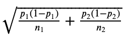
Finally, the confidence interval is (point_estimate ± critical_value X standard-error) , or:
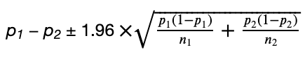
Let’s plug our numbers into these formulas, using some helper functions to do so.
Finally, the calc_ci_range function puts everything together.
Let's calculate the confidence intervals for our leaning groups, looking first at left vs. right.
Looking at the difference in proportions for left vs right publications, our confidence interval ranges from 1.8% to 2.1%. This is both a fairly narrow range and far from zero relative to the overall range of the difference in proportion. So rejecting the null hypothesis is obvious. Similarly, the range for center vs left is 1.3% to 2.1%:
Because the assignment of publications to bias slant is somewhat subjective, here is another variant, putting Business Insider, NY Post, and NPR in center .

Next, we can look at publication ownership, using the same approach. We divide our population into four groups, LLC, corporation, non-profit, and private.
Now let's plot that data to see whether different types of companies cover climate change in different proportions.

Perhaps unsurprisingly, it looks like private companies and nonprofits cover climate change a bit more than corporations and LLCs. But let's look more closely at the difference in proportion between the first two, LLCs and corporations:
Here, the confidence interval is 0.3% to 0.7%, much closer to zero than our earlier differences, but still not including zero. We would expect the non-profit to LLC interval to also not include zero:
The non-profit to LLC confidence interval is 0.6% to 1.2%.Finally, looking at private vs. non-profit, we find a confidence interval of -0.3% to 0.5%:
Thus in this case, we can conclude that there is not a significant difference in proportion of climate change related articles between these two populations, unlike the others populations we’ve compared.
Summary: Text Analysis to Test a Hypothesis
In this article, we've performed some text analysis on a large corpus of news articles and tested some hypotheses about the differences in their content. Specifically, using a 95% confidence interval, we estimated differences in climate change discussions between different groups of news sources.
We found some interesting differences which were also statistically significant, including that right-leaning news sources tend to cover climate change less, and corporations and LLCs tend to cover it less than non-profit and private outlets.
In terms of working with this corpus, though, we've barely touched the tip of the iceberg. There are many interesting analyses you could attempt with this data, so download the data from Kaggle for yourself and start writing your own text analysis project!
Further Reading:
Olteanu, A, et al. “Comparing events coverage in online news and social media: The case of climate change.” Proceedings of the Ninth International AAAI Conference on Web and Social Media. 2015.
More learning resources
Math in data science, tutorial: basic statistics in python — descriptive statistics.
Learn data skills 10x faster

Join 1M+ learners
Enroll for free
- Data Analyst (Python)
- Gen AI (Python)
- Business Analyst (Power BI)
- Business Analyst (Tableau)
- Machine Learning
- Data Analyst (R)
- Welcome to Hypothesis!
- Edit on GitHub
Welcome to Hypothesis! 
Hypothesis is a Python library for creating unit tests which are simpler to write and more powerful when run, finding edge cases in your code you wouldn’t have thought to look for. It is stable, powerful and easy to add to any existing test suite.
It works by letting you write tests that assert that something should be true for every case, not just the ones you happen to think of.
Think of a normal unit test as being something like the following:
Set up some data.
Perform some operations on the data.
Assert something about the result.
Hypothesis lets you write tests which instead look like this:
For all data matching some specification.
This is often called property-based testing, and was popularised by the Haskell library Quickcheck .
It works by generating arbitrary data matching your specification and checking that your guarantee still holds in that case. If it finds an example where it doesn’t, it takes that example and cuts it down to size, simplifying it until it finds a much smaller example that still causes the problem. It then saves that example for later, so that once it has found a problem with your code it will not forget it in the future.
Writing tests of this form usually consists of deciding on guarantees that your code should make - properties that should always hold true, regardless of what the world throws at you. Examples of such guarantees might be:
Your code shouldn’t throw an exception, or should only throw a particular type of exception (this works particularly well if you have a lot of internal assertions).
If you delete an object, it is no longer visible.
If you serialize and then deserialize a value, then you get the same value back.
Now you know the basics of what Hypothesis does, the rest of this documentation will take you through how and why. It’s divided into a number of sections, which you can see in the sidebar (or the menu at the top if you’re on mobile), but you probably want to begin with the Quick start guide , which will give you a worked example of how to use Hypothesis and a detailed outline of the things you need to know to begin testing your code with it, or check out some of the introductory articles .
- Stack Overflow for Teams Where developers & technologists share private knowledge with coworkers
- Advertising & Talent Reach devs & technologists worldwide about your product, service or employer brand
- OverflowAI GenAI features for Teams
- OverflowAPI Train & fine-tune LLMs
- Labs The future of collective knowledge sharing
- About the company Visit the blog
Collectives™ on Stack Overflow
Find centralized, trusted content and collaborate around the technologies you use most.
Q&A for work
Connect and share knowledge within a single location that is structured and easy to search.
Get early access and see previews of new features.
Generate random data for testing a pandas dataframe with hypothesis
I am working a lot of pandas dataframes and I want to test them using pytest and I am using hypothesis to generate the test data.
The issues I am having is that it is generating the same data values in each column.
I actually don't know how to generate real data to test with ..
Here is what I am trying :
this is always generating the following dataset
And as you can see for that each colunms have one values not unique values , I don't know how to generate real values I can test with ..
Any help will be helpful...
- python-hypothesis
- Thank for this commentt , I thought about that but the issues is that those dates should not be unique – Espoir Murhabazi Commented Jan 13, 2021 at 20:08
2 Answers 2
Zac gives some good insight in his answer and from that, I understood why I was getting the issue, I managed to have some data with the code I shared with some hack from the documentation. Although it is not generating 100% of what I wanted it was enough for the testing.
Here is how I generated the columns and afterward the data.
I use the following code to define the columns strategies :
Then I created the dataframes with :
Next I generated my dataset with :
And finally, I was able to run the following tests
Note the min_size in the index from the dataset generation and the max_example in the settings.
The first example is because Hypothesis always starts by generating the simplest possible example , which will be all-zeros (etc.). I'd recommend turning up the max_examples setting - the default 100 is good, but less than 20 is very very few.
You've also specified a very large min_size=100 for your index - is it really impossible to have a failing example with fewer rows? If not, set it much smaller - Hypothesis is great a finding bugs with small inputs, and they're way faster to generate too.
Completing our set of causes, Hypothesis generates dataframes with a "fill value" for each column - and at this large size and few examples, when you only see the first few and last few rows all you're looking at is the minimal fill-value. Set min_size=1 and this problem will go away entirely.
- 1 Thanks @zac for this .. I think I am getting what I was missing let me implement it and I will tell you how it goes – Espoir Murhabazi Commented Jan 14, 2021 at 10:40
Your Answer
Reminder: Answers generated by artificial intelligence tools are not allowed on Stack Overflow. Learn more
Sign up or log in
Post as a guest.
Required, but never shown
By clicking “Post Your Answer”, you agree to our terms of service and acknowledge you have read our privacy policy .
Not the answer you're looking for? Browse other questions tagged python pandas python-hypothesis or ask your own question .
- The Overflow Blog
- One of the best ways to get value for AI coding tools: generating tests
- The world’s largest open-source business has plans for enhancing LLMs
- Featured on Meta
- User activation: Learnings and opportunities
- Site maintenance - Mon, Sept 16 2024, 21:00 UTC to Tue, Sept 17 2024, 2:00...
- Staging Ground Reviewer Motivation
- What does a new user need in a homepage experience on Stack Overflow?
Hot Network Questions
- The quest for a Wiki-less Game
- Example of two dinatural transformations between finite categories that do not compose
- What was the main implementation programming language of old 16-bit Windows versions (Windows 1 - Windows 3.11)?
- O(nloglogn) Sorting Algorithm?
- Kotlin object expression property scope and shadowing rules
- Were the PS5 disk version console just regular digital version consoles with a pre-installed disk module?
- Why is the area covered by 1 steradian (in a sphere) circular in shape?
- "Tail -f" on symlink that points to a file on another drive has interval stops, but not when tailing the original file
- How can I stop the noise from updating its position when I adjust the spline?
- Why are my empty files not being assigned the correct mimetype?
- How would platypus evolve some sort of digestive acid?
- How much technological progress could a group of modern people make in a century?
- Is a thing just a class with only one member?
- What came of the Trump campaign's complaint to the FEC that Harris 'stole' (or at least illegally received) Biden's funding?
- What is meant by applying operator to a function?
- How can I analyze the anatomy of a humanoid species to create sounds for their language?
- Attacks exploiting decryption failures in KYBER
- Should I write an email to a Latino teacher working in the US in English or Spanish?
- cat file contents to clipboard over ssh and across different OS
- A journal has published an AI-generated article under my name. What to do?
- Where to put acknowledgments in a math paper
- Can Cantrip Connection be used with innate cantrips?
- Does hydrogen peroxide work as a rocket fuel oxidizer by itself?
- Why did early ASCII have ← and ↑ but not ↓ or →?
Member-only story
Hypothesis and Pandera: Generate Synthesis Pandas DataFrame for Testing
Create clean and robust tests with property-based testing.
Khuyen Tran
Towards Data Science
Imagine you are trying to figure out whether the function processing_fn is working properly. You use pytest to test the function with an example.
The test passed, but you know that one example is not enough. You need to test the function with more examples to make sure that the function is working properly with any data.

Written by Khuyen Tran
MLOps Engineer. Website: https://mathdatasimplified.com
Text to speech
Sign up for a free recipe e-book →
Python Libraries for Data Analysis: Pandas and NumPy
Published by

In today’s data-driven world, analyzing and interpreting large volumes of information is crucial for making informed decisions. Python, a versatile programming language, has become a favorite tool for data analysis, largely due to its powerful libraries. Among these, Pandas and NumPy stand out as essential tools. If you’re new to data analysis or looking to sharpen your skills, understanding these libraries is a great place to start.
What is NumPy?
NumPy, short for Numerical Python, is a foundational library in Python for numerical computing. It provides support for arrays, which are more efficient than Python’s built-in lists for large datasets. This efficiency is crucial for performing complex calculations and data manipulation quickly.
Key Features of NumPy:
- Arrays: NumPy’s core feature is its multi-dimensional array object, ndarray. Unlike lists, arrays can be multi-dimensional, which means they can handle matrices and higher-dimensional data structures effectively. Arrays support element-wise operations, making them ideal for mathematical computations.
- Mathematical Functions: NumPy offers an extensive array of mathematical functions, including trigonometric operations, statistical calculations, and linear algebra routines.These functions are optimized for performance, making complex calculations faster and more efficient.
- Broadcasting: This powerful feature allows NumPy to perform operations on arrays of different shapes in a way that avoids unnecessary data duplication and increases computational efficiency.
- Integration with Other Libraries: NumPy integrates seamlessly with other scientific computing libraries like SciPy and scikit-learn, enhancing its functionality and making it easier to conduct more advanced analyses.
What is Pandas?
Pandas is another essential library for data analysis in Python. It provides high-level data structures and methods designed to work with structured data. If you’ve ever worked with data in spreadsheets or databases, you’ll find Pandas’ DataFrame object familiar and easy to use.
Key Features of Pandas:
- DataFrames: The main data structure in Pandas is the DataFrame, which resembles a table in a database or an Excel spreadsheet. DataFrames allow you to store and manipulate tabular data in a straightforward way, with labeled axes (rows and columns).
- Series: Series: A Series is a one-dimensional, array-like object that can store any data type. It essentially represents a single column within a DataFrame. Series objects are useful for handling and analyzing individual columns of data.
- Data Manipulation: Pandas offers powerful tools for data manipulation, such as filtering, grouping, merging, and reshaping data. These capabilities make it easy to clean and transform data before analysis.
- Handling Missing Data: Missing data is a common issue in real-world datasets. Pandas provides methods for detecting, filling, and interpolating missing values, making it easier to prepare data for analysis.
- Time Series Analysis: Pandas has robust support for time series data, which is crucial for financial data analysis, forecasting, and any analysis involving dates and times.
How Pandas and NumPy Work Together
While NumPy and Pandas serve different purposes, they are often used together in data analysis workflows. Here’s how they complement each other:
- Data Storage and Computation: NumPy arrays are used for numerical computations and can be the foundation for more complex data structures. Pandas DataFrames, on the other hand, use NumPy arrays to store their data but provide additional functionality for data manipulation and analysis.
- Performance Optimization: NumPy’s array operations are optimized for performance and are used internally by Pandas. When you perform operations on a DataFrame, Pandas often leverages NumPy for the underlying computations.
- Interoperability: You can easily convert between Pandas DataFrames and NumPy arrays, allowing you to use NumPy’s computational power and Pandas’ data manipulation capabilities interchangeably.
Practical Applications
- Data Cleaning: Pandas makes it easy to clean and preprocess data by handling missing values, removing duplicates, and transforming data types. NumPy assists in performing calculations and transformations on large datasets.
- Exploratory Data Analysis (EDA): EDA involves summarizing and visualizing data to uncover patterns and insights. Pandas provides functions for summarizing data, calculating statistics, and plotting basic charts, while NumPy helps in performing more complex mathematical operations.
- Statistical Analysis: Both libraries support statistical analysis, but Pandas offers higher-level abstractions for working with data, such as rolling statistics and resampling, whereas NumPy provides lower-level mathematical functions.
- Machine Learning: For machine learning tasks, you often start with data preprocessing using Pandas and then perform numerical computations and model building with NumPy. Many machine learning libraries in Python are built on top of NumPy.
Getting Started with Pandas and NumPy
To start using Pandas and NumPy, you need to install these libraries, typically via a package manager like pip. Once installed, you can import them into your Python script or notebook. From there, you can begin loading data, performing computations, and exploring the extensive functionalities offered by both libraries.
Key Points to Remember:
- NumPy is best for numerical operations and handling large arrays of data efficiently.
- Pandas is ideal for working with structured data, including data cleaning, manipulation, and analysis.
- The two libraries work well together, with Pandas often using NumPy arrays for its underlying data structures and computations.
Pandas and NumPy are indispensable tools in the data analyst’s toolkit. While NumPy provides the foundation for numerical operations and efficient array handling, Pandas offers a higher-level interface for working with structured data. Understanding how to leverage both libraries can significantly enhance your data analysis capabilities, allowing you to handle everything from basic data manipulation to complex statistical analysis and machine learning tasks. By mastering Pandas and NumPy, you’ll be well-equipped to tackle a wide range of data analysis challenges. To deepen your expertise, you might explore Data Analytics course in Lucknow , Nagpur, Delhi, Noida, and other prominent locations across India. These courses offer comprehensive training in both Pandas and NumPy, alongside other essential data analysis skills.
Share this:
Leave a comment cancel reply, i'm emily.

Welcome to Nook, my cozy corner of the internet dedicated to all things homemade and delightful. Here, I invite you to join me on a journey of creativity, craftsmanship, and all things handmade with a touch of love. Let's get crafty!
Let's connect
Join the fun.
Stay updated with our latest tutorials and ideas by joining our newsletter.
Type your email…
Recent posts

How to Implement Shift-Left Testing in Your Development Cycle

Why Data Science? Understanding Its Role in Modern Business

A Comprehensive Guide to OWASP ZAP and Burp Suite: Essential Tools for Security Testing

Data Science Primer: From Basics to Advanced

Understanding Automation Frameworks: Design and Implementation
- Already have a WordPress.com account? Log in now.
- Subscribe Subscribed
- Copy shortlink
- Report this content
- View post in Reader
- Manage subscriptions
- Collapse this bar
MDF4 Files to CSV: handling Automotive data easily with Python and Open-Source tools
Let me show you how I use open-source Python libraries to handle MDF files from Automotive testing and calibration environments

Luis Medina
Using asammdf api and pandas to handle automotive asam data.
Let me show you an example of how you can parse MDF4 or other ASAM files and convert them to common formats.
Traditionally, the tools you'd need to process this type of file were only accessible through expensive licenses, like ETAS MDA , or Matlab's Vehicle Networks Toolbox to cite some commonly known examples. However, CSS electronic s has done a great job at releasing and maintaining a Python-friendly asammdf API , which is an excellent free and open-source alternative.
What are MDF4 files?
MDF4 files are commonly used in the Automotive Industry for software development, calibration, and testing data. It is the most recent evolution of the original MDF file, developed in the 90's by Vector Informatik GmbH and Robert Bosch GmbH.
MDF stands for Measurement Data Format. Nowadays, it is defined by the ASAM (Association of Standardization of Automation and Measurement Systems) in the ASAM MDF standard .
ASAM MDF files are very useful for Automotive measurement and calibration data, because they can efficiently store large amounts of data, retaining information about the communication and acquisition systems used to create them, while being very fast to query and index.
The problem with them is that, unlike .csv or ASCII files, you can't just load them and preprocess them with Data Visualization tools, like Tableau, Power BI or more IoT-oriented ones, like Grafana. To handle them, you first need to convert them to a more manageable format, and this what I'm going to show, using asammdf and Python.
Taming the beast they don't tell you about in your Data Analytics online course
This is an industry-specific and tightly packed type of animal you probably never heard about while learning about data analytics until you decided to work for an Automotive company or a service provider for those companies.
Fortunately, converting MDF4 files to a more manageable format is easier than you'd think - in most cases.
Here's the barebones version of the code I'd use:
And there it is, a CSV file you can work with following most online tutorials about data visualization 101.
I hope you found this useful and feel free to copy-paste it for your own projects. Please do read the official documentation of this API so you know what you are doing, though.
I still have some words about the choices you'll have to make when working with Automotive data. You might want to stick around and keep reading, especially if you aren't familiar with the Automotive testing and calibration area.
Why use a signal list?
Using asammdf API we can easily import all the signals contained within an input ASAM file. However, in my experience, when preparing data for a visualization pipeline, you likely won't want to include all the signals available.
In Automotive software (and therefore in data coming from Automotive Networks, logged in ASAM MDF formats), it's common to have tens, or even hundreds of signals containing error flags, status values, and other information you might not need. Software developers need them, Application Engineers need them, but you, as a Data Analytics expert, don't.
If you are working on a project that requires you to look at some of those, then, by all means, include them. But in most cases, you don't want to visualize them all.
Of course, it depends on what you are trying to achieve, so there isn't a definitive solution here. My suggestion is, import only the channels you'll actually use.
Something interesting about the list of signals is that it can act as additional documentation about what information you are using. They could be descriptive - literally including a description for each signal, like this:
- You might need to over-complicate your workflow just to get the description from the raw MDF4 file.
- When you do so, it's very possible that the signals you are ingesting don't have an associated description, of the description is cryptic and hard to understand (sometimes even cryptic AND in a different language because you are logging signals from a component from a foreign supplier).
That is why, in my opinion, you should always contact the function experts or system engineers and align with them about what information is carried by the signals you are using.
What about the sampling rates?
Whether to choose a unique sampling rate to apply to all your signals or not is a decision you'll have to make by having a good understanding of the data you are using, what it represents and what the visualization is going to be used for. What do you or the stakeholders want to achieve by visualizing these data?
Looking at short-term events: rapidly-varying, dynamic phenomena
If you are visualizing data to analyze in detail something that happened over a short period (minutes, hours) you might want to look at the short-term trends or patterns in your signals.
Maybe you need to analyze when a failure happened, so you need to see signals varying rapidly and perhaps identify the instant when the system you are looking at reacted in some way. This could mean you need to visualize signals sampled at 10 Hz or more. Common Automotive ECUs have different task rates, such as 1000 ms, 100 ms, 10 ms and sometimes even 1 ms or faster.
In that case, you might want to retain each signal with its associated raster, so you can look at the information as it was logged by the system, with it's "native" sampling time, especially if you need to look at the details of a 2-second phenomena, for instance.
The drawback of doing this, is that you'll need to include both each signal and its sampling time in your analyses, meaning that there won't be a single time base that you can use to visualize timeseries data.
Another approach would be to re-sample all signals to match the highest sampling rate among the signals you'll need to visualize. That way, you don't crop any information, and you get to work with a single time base. In this case, you'll end up with too many samples so your workflow might get slowed down.
In my case, I always strive for a trade-off between the number of channels (signals) I need to look at, and the fastest phenomena I need to observe. As with all things engineering-related: do not lose or crop the information your stakeholders will actually want to look at.
Looking at longer-term events: trends and patterns over longer periods of time
Another common scenario - one in which you might want to use a data pipeline and create a visualization dashboard - is when you need to look at phenomena that change slowly over time.
For example, the temperature trends over several days, or weeks. In that case, it makes sense to re-sample everything to a lower frequency, because you don't care about the high-frequency information in your data. Why would you plot a signal that has 100 samples per second (100 Hz) when you need to look at several weeks? By resampling, you can reduce the amount of data you have to work with, without losing the information you care about.
Why convert to Pandas Dataframes?
With asammdf API , exporting an .MF4 file as .csv is straightforward simply using the MDF.export('csv') method. So converting to a Pandas data frame first seems like an unnecessary step.
In my opinion, having a Pandas Dataframe lets you use all the great functionalities of Pandas to pre-process your data before you plot it, export it, or write it to a database.
If you are interested in learning more about Pandas , a good place to start is the Pandas & Python for data analysis full course by FreeCodeCamp , and there are many tutorials in video and text formats online. I've also written a few articles where show things I've found interesting about it, so might want to check them out.
This example shows a manual workflow to open and visualize the data within an MDF4 file, and export it as a .CSV. The idea is to showcase the basic usage of ASAMMDF API for local conversion and analysis.
If you want to automate this to deploy it at a larger scale, you'll need to integrate some of this in your pipeline and handle file selection and import more efficiently, and consider not exporting the data as a file, but instead writing it to a database that you can query.
This subject is interesting for me, because I'm an Engineer working in Automotive/Heavy Duty Embedded Software, but I'm also a data nerd. I hope this was useful to people wanting to work with MDF4 files without having access to industry-standard tools and licenses.
Nowadays, I feel like converting MDF files to different formats using non-proprietary tools will become more and more common, as Automotive OEMs start hiring more people for Data Analytics positions, and more companies start to offer Analytics services for the Automotive sector.
Also, companies aiming at creating Digital Twins can use open-source tools like these to leverage the capabilities of Cloud Computing and microservices to handle their MDF data - think a Python script running on a cloud instance, versus a Matlab script for which you need a license.
That's another good reason for replacing Matlab with Python in your workflow.
Using Autodesk Fusion's flat pattern feature
I share my workflow on Autodesk Fusion to export flattened surfaces for laser cutting
Leveraging data aggregations in Python: using Pandas groupby method for data analysis
I share the intuition that helped me understand Pandas GroupBy method and examples of how it can be so useful when analyzing data.
DL Notes: Advanced Gradient Descent
I researched the main optimization algorithms used for training artificial neural networks, implemented them from scratch in Python and compared them using animated visualizations.
DL Notes: Gradient descent
I describe the algorithm of gradient descent, which is used to adjust the weights of an ANN. A summary of information from different sources that I used when studying this topic.
COMMENTS
It tests the null hypothesis that the population variances are equal (called homogeneity of variance or homoscedasticity). Suppose the resulting p-value of Levene's test is less than the significance level (typically 0.05).In that case, the obtained differences in sample variances are unlikely to have occurred based on random sampling from a population with equal variances.
Example 1: One Sample t-test in Python. A one sample t-test is used to test whether or not the mean of a population is equal to some value. For example, suppose we want to know whether or not the mean weight of a certain species of some turtle is equal to 310 pounds. To test this, we go out and collect a simple random sample of turtles with the ...
In this post, you will discover a cheat sheet for the most popular statistical hypothesis tests for a machine learning project with examples using the Python API. Each statistical test is presented in a consistent way, including: The name of the test. What the test is checking. The key assumptions of the test. How the test result is interpreted.
A hypothesis test evaluates two mutually exclusive statements about a population to determine which ... (python code is below for same) one-sample Z test. import pandas as pd from scipy import stats from statsmodels.stats import weightstats ... check example in python below. df_chi = pd.read_csv('chi-test.csv') contingency_table=pd.crosstab(df ...
Paired T-Test with Pandas. ... I hope this end-to-end look at hypothesis testing methodology, Python programming demonstrations, real-world grounding, inherent restrictions and next level considerations provides a launchpad for practically applying core statistics! Please subscribe using the form below for more data science tutorials.
Dive into the fascinating process of hypothesis testing with Python in this comprehensive guide. Perfect for aspiring data scientists and analytical minds, learn how to validate your predictions using statistical tests and Python's robust libraries. From understanding the basics of hypothesis formulation to executing detailed statistical analysis, this article illuminates the path to data ...
Master hypothesis testing with Python: Learn statistical validation and data-driven decision-making in a concise guide. ... In Python, we can use libraries like Pandas and Numpy to calculate the ...
Image by Author. We use the boxplot() pandas function to create box plots for the compactness variable. Evidently, the Kama and Rosa varieties have similar quartiles, with median values that are nearly identical. In contrast, the Canadian variety appears to slightly differ from the rest, but we need to verify this with a hypothesis test.
import numpy as np import scipy.stats as stats import pandas as pd import matplotlib.pyplot as plt 4. Hypothesis Testing in Python: Examples Example 1: One Sample T-test. One sample T-test is used when we want to compare the mean of a population to a specified value. For example, let's consider a scenario where we want to test if the average ...
Before we can start any hypothesis testing, ensure you have Python installed along with the necessary libraries. For this tutorial, we'll be using pandas, scipy, and matplotlib.
In this article, we interactively explore and visualize the difference between three common statistical tests: t-test, ANOVA test and Chi-Squared test. We also use examples to walk through essential steps in hypothesis testing: 1. define the null and alternative hypothesis. 2. choose the appropriate test.
Example 1: Independent Two Sample t-Test in Pandas. An independent two sample t-test is used to determine if two population means are equal. For example, suppose a professor wants to know if two different studying methods lead to different mean exam scores. To test this, he recruits 10 students to use method A and 10 students to use method B.
Hypothesis Testing in Python. In this course, you'll learn advanced statistical concepts like significance testing and multi-category chi-square testing, which will help you perform more powerful and robust data analysis. Enroll for free. Part of the Data Analyst (Python), and Data Scientist (Python) paths. 4.8 (359 reviews)
The pandas data-frame; Hypothesis testing: comparing two groups. Student's t-test: the simplest statistical test; ... from the pandas module. It is the Python equivalent of the spreadsheet table. ... Hypothesis testing and p-values give you the significance of an effect / difference.
Hypothesis Testing using Python. Aman Kharwal. March 25, 2024. Machine Learning. 1. Hypothesis Testing is a statistical method used to make inferences or decisions about a population based on sample data. It starts with a null hypothesis (H0), which represents a default stance or no effect, and an alternative hypothesis (H1 or Ha), which ...
At the same time, we'll learn some of the programming skills required to analyze text data in Python and test a hypothesis related to that data. This tutorial assumes that you're fairly familiar with Python and the popular data science package pandas. If you'd like to brush up on pandas, check out this post, ...
Welcome to Hypothesis! Hypothesis is a Python library for creating unit tests which are simpler to write and more powerful when run, finding edge cases in your code you wouldn't have thought to look for. It is stable, powerful and easy to add to any existing test suite. It works by letting you write tests that assert that something should be ...
Statistical tests are used in hypothesis testing. In general, they can be used to: determine whether an input variable has a statistically significant relationship with an output (target) variable. ... an open-source statistical package written in Python 3 and based mostly on Pandas and NumPy. Scipy: a Python-based ecosystem of open-source ...
H1: There is a relationship between hot weather (greater than 28 degrees Celsius) and the number of car accidents. I am not sure of how to calculate the p-value for the above hypothesis in python. I did the following: import pandas as pd. from scipy.stats import ttest_ind.
3. I am trying to run a hypothesis test using model ols. I am trying to do this model Ols for tweet count based on four groups that I have in my data frame. The four groups are Athletes, CEOs, Politicians, and Celebrities. I have the four groups each labeled for each name in one column as a group. frames = [CEO_df, athletes_df, Celebrity_df ...
The first example is because Hypothesis always starts by generating the simplest possible example, which will be all-zeros (etc.).I'd recommend turning up the max_examples setting - the default 100 is good, but less than 20 is very very few.. You've also specified a very large min_size=100 for your index - is it really impossible to have a failing example with fewer rows?
Something went wrong and this page crashed! If the issue persists, it's likely a problem on our side.
Explore and run machine learning code with Kaggle Notebooks | Using data from multiple data sources
Pandera is a simple Python library for validating a pandas DataFrame. Validate Your pandas DataFrame with Pandera. Make Sure Your Data Matches Your Expectation. ... Hypothesis — Create Examples for Testing. Next, we will use hypothesis to create data for testing based on the constraints given by pandera.DataFrameSchema. Specifically, we will add:
In today's data-driven world, analyzing and interpreting large volumes of information is crucial for making informed decisions. Python, a versatile programming language, has become a favorite tool for data analysis, largely due to its powerful libraries. Among these, Pandas and NumPy stand out as essential tools. If you're new to data analysis or looking to…
Why convert to Pandas Dataframes? With asammdf API, exporting an .MF4 file as .csv is straightforward simply using the MDF.export('csv') method. So converting to a Pandas data frame first seems like an unnecessary step. In my opinion, having a Pandas Dataframe lets you use all the great functionalities of Pandas to pre-process your data before you plot it, export it, or write it to a database.